How to Needlessly Produce Inflation

 

John P. Hussman, Ph.D.
President, Hussman Investment Trust

August 2019

---

I’ve noted over the years that substantial market declines are often preceded by a combination of internal dispersion, where the market simultaneously registers a relatively large number of new highs and new lows among individual stocks, and a leadership reversal, where the statistics shift from a majority of new highs to a majority of new lows within a small number of trading sessions.
-John P. Hussman, Ph.D.
Market Internals Go Negative, July 30, 2007

What distinguishes an overvalued market that continues to advance from an overvalued market that often drops like a rock? In my view, it’s the psychological disposition of investors toward speculation or risk-aversion. Though investor psychology seems abstract and intangible, it can also be inferred from market action. Speculation tends to be indiscriminate, and the strongest market advances are typically also the broadest. In contrast, risk-aversion gradually reveals itself in divergences, dispersion, and eventually ragged market action and disorder.

As a result, we find that the best measure of that investor psychology is the uniformity or divergence of market action across thousands of individual securities, industries, sectors, and security-types, including debt securities of varying creditworthiness. I use the word “market internals” to describe the signal we extract from their joint behavior across multiple facets, including trend, momentum, trading volume, leadership, yield spreads, breadth, participation, and other metrics.

Two weeks ago, I posted a special interim update to our website and mailing list, They’re Running Toward the Fire, noting “Presently, we observe market conditions that have been associated almost exclusively, and in most cases precisely, with the most extreme bull market peaks across history.”

That concern reflects not only hypervaluation on the measures we find best correlated with long-term market returns, but also unfavorable market internals, the emergence of single most extreme “overvalued, overbought, overbullish” syndrome we identify, and features of breadth (advancing issues vs. declining issues) and leadership (new highs vs. new lows) that often accompany market extremes.

Market valuations have been extreme for a long time. While valuations have enormously important implications for long-term market returns and full-cycle market risks, valuations are not a timing tool. Indeed, it’s impossible for the market to reach hypervalued levels without persistently advancing through lesser extremes. It’s the combination of extreme valuations, plus unfavorable market internals (indicating a shift among investors from speculation toward risk-aversion), plus extreme overextension, plus dispersion and reversals in leadership, that create a volatile mix.

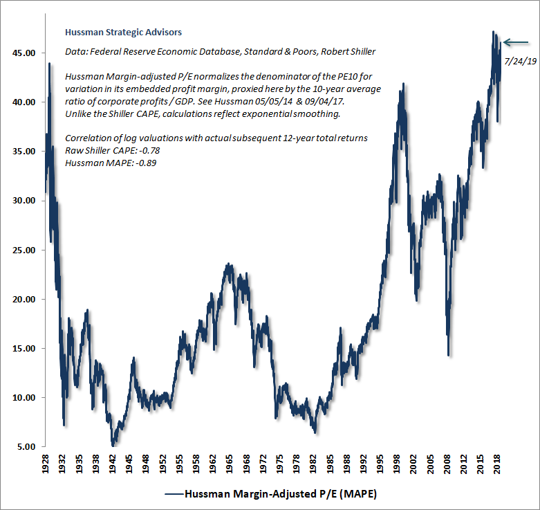
A quick review of these conditions will suffice. The following chart shows our Margin-Adjusted P/E for the S&P 500 Index, which is better correlated with actual subsequent market returns than a wide range of alternatives, including price/forward-earnings, the Shiller cyclically-adjusted P/E (CAPE), and the so-called Fed Model (the S&P 500 forward earnings yield vs. 10-year Treasury yields).

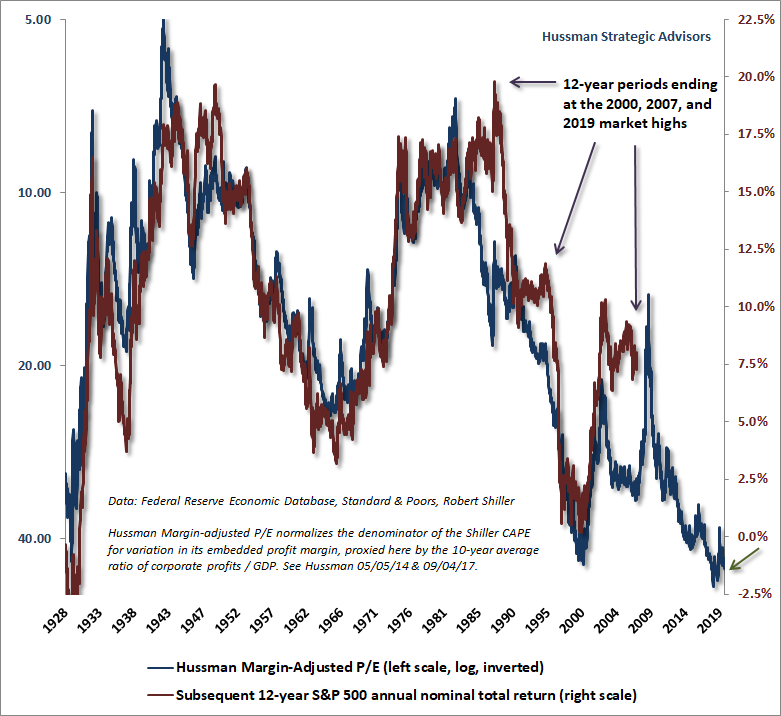
The next chart presents the relationship between the Margin-Adjusted P/E, shown here on an inverted log scale on the left, with actual subsequent 12-year S&P 500 total returns, shown on the right scale. You’ll notice a few points where the actual return of the S&P 500 over a given 12-year horizon diverges from the return that one would have expected years earlier, based on market valuations alone. Those divergences are a hallmark of bubbles. Again, it’s impossible for the market to reach hypervalued extremes without a period in which it has persistently advanced through lesser extremes.

Understand that low interest rates don’t “justify” these hypervalued extremes. When Wall Street analysts make this argument, what they are really saying is that interest rates are terribly low, so stocks should be priced at valuations that ensure terribly low future equity returns as well. But the situation is even worse, because the structural growth rate of the U.S. economy (labor force growth plus trend productivity) is only about 1.6% at present, versus growth of over 3% annually for much of the post-war period before 2000.

That low level of structural growth is why nominal S&P 500 revenues have grown at just 3.7% annually over the past 20 years, including the impact of share buybacks. That compares to an average post-war growth rate of about 6.5%. Earnings have grown somewhat faster than revenues during this period due to expansion in profit margins from historically below-average levels to historical extremes, but unless one expects profit margins to expand without limit, even permanently high profit margins would result in future earnings growth being roughly the same as future revenue growth.

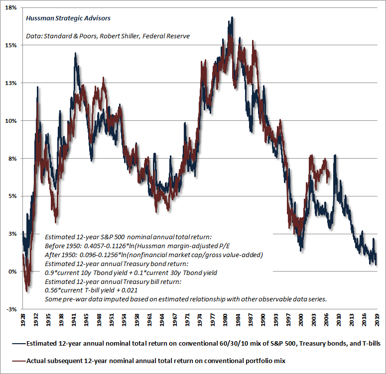
The problem is that if interest rates are low because growth is also low, then no valuation premium is “justified” at all. In that situation, rich valuations merely add insult to injury. Notably, our estimates for future S&P 500 market returns do not reflect any downward adjustment for lower growth rates, so my sense is that they may actually be a bit optimistic. Still, at the end of July, our estimate of prospective 12-year total returns for a conventional asset mix invested 60% in the S&P 500, 30% in Treasury bonds, and 10% in Treasury bills, reached the lowest level in history except for the single week of the August 1929 market top.

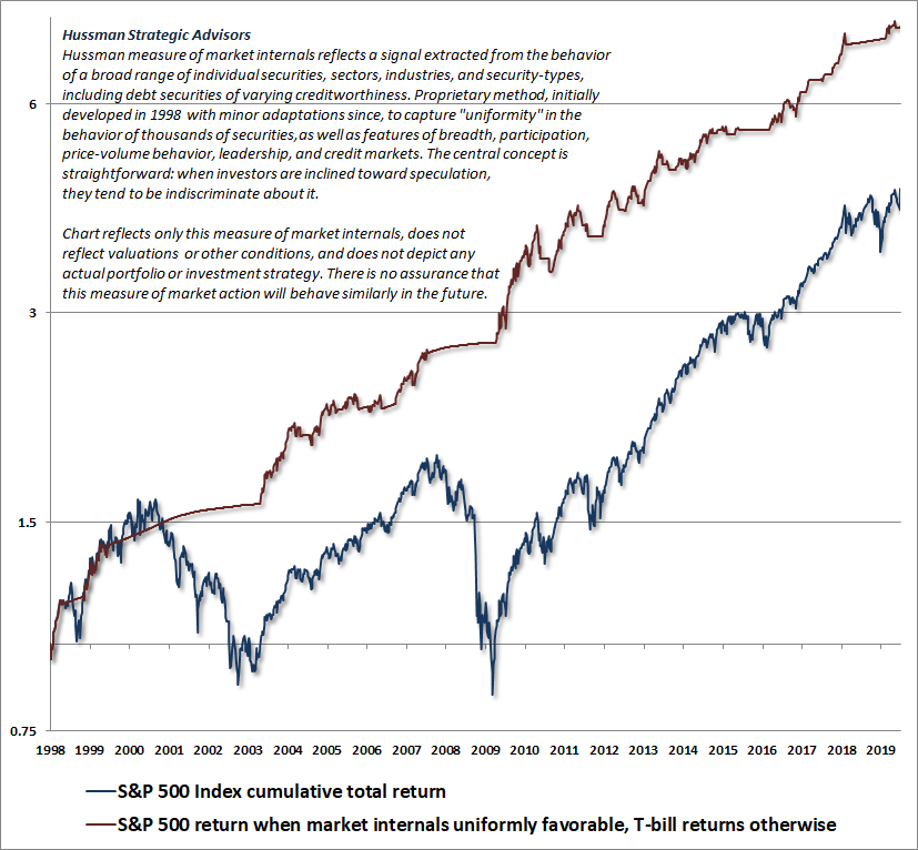
This brings us to internals. The chart below shows the cumulative total return of the S&P 500 since 1998, when I first introduced market internals into our discipline, along with the cumulative total return of the S&P 500 restricted only to those periods where market internals are favorable on our measures (accumulating Treasury bill returns otherwise). The chart is historical, does not reflect the performance of any portfolio, and there is no assurance that future market returns will be similarly related to these measures. Those of you who have been with me across multiple cycles know that the uniformity and divergence of market internals was critical for us in anticipating the collapses of 2000-2002 and 2007-2009.

As I’ve detailed before, our difficulty in the advancing half-cycle since 2009 had nothing to do with valuations or market internals, but instead on my pre-emptive bearish response to “overvalued, overbought, overbullish” extremes that had historically placed well defined limits to speculation, and were regularly followed by air-pockets, panics, or crashes in previous market cycles.

In late-2017, I abandoned the idea that yield-seeking speculation had “limits” in the face of the Federal Reserve’s policies of quantitative easing and zero interest rates. Instead, we resolved to refrain from adopting or amplifying a negative market outlook except when our measures of market internals have also explicitly deteriorated. That adaptation is the key change that would have allowed our experience in the recent half- cycle to more closely mirror the experience of our investment discipline in complete cycles prior to 2009.

Our measures of internals shifted negative on February 2, 2018, and with very brief exception, have remained unfavorable since. Notably, at the close of Friday, August 2, 2019, the S&P 500 Index stood within about 2% of both its January 2018 and September 2018 pre-correction peaks.

The period of negative internals since February 2018 has resulted in a sideways market with multiple V-shaped corrections. Ironically, the main challenge for hedged-equity approaches since then has been the internal dispersion of the market itself. It has been difficult for broad stock selection approaches, particularly value-conscious ones, to gain traction versus the capitalization-weighted S&P 500 Index.

Here’s what’s going on. While increasing risk-aversion at hypervalued extremes typically results in spectacular market losses, the dispersion since early-2018 has been accompanied by a price-insensitive and backward-looking exodus of investors toward passive indexing, despite the highest valuations and weakest prospective market returns since the 1929 peak. Indeed, Morningstar reports that nearly half of all mutual fund assets are now passively managed, typically tied to capitalization-weighted indices like the S&P 500. All of this backward-looking performance chasing is likely to end badly, but over the short-run, it has been a thorn in the side of value investors.

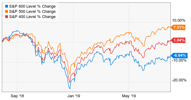
The chart below offers a bit of perspective on the recent divergence between the large capitalization-weighted S&P 500, and broad indices of mid-cap (S&P 400) and small-cap (S&P 600) stocks (h/t Mike Shell).

There’s no question that my pre-emptive bearish response to increasingly extreme “overvalued, overbought, overbullish” syndromes was detrimental in this half-cycle, and there’s no question that prioritizing internals – as we have did in late-2017 – would have vastly improved our experience. Regardless of how extreme valuations may be, whenever our measures of market internals become favorable, we will shift toward a neutral or constructive near-term outlook and defer our expectations for immediate market losses.

Having admirably navigated decades of complete market cycles prior to 2009, there are some who nonetheless confuse a hypervalued market with intelligence, and take a certain delight in my error in the recent half-cycle, as if I’ve neither admitted nor addressed it. They seem to harbor the mistaken idea that a hypervalued market can be ignored even when ragged internals indicate a shift toward risk-aversion among investors. Can’t say I haven’t warned them.

Presently, we observe market conditions that have been associated almost exclusively, and in most cases precisely, with the most extreme bull market peaks across history.

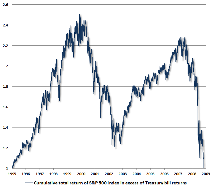
Meanwhile, it’s also useful to remember how forgiving the complete market cycle is of exiting an overvalued market too early. The fact is that the 2000-2002 collapse wiped out every bit of total return that the S&P 500 had accrued over-and-above T-bills, all the way back to May 1996. The 2007-2009 collapse did the same, all the way back to June 1995.

The chart below shows how the temporary benefits of multiple valuation bubbles can be wiped out over the completion of a market cycle. Presently, a retreat in valuations, to the highest level ever observed at the end of any market cycle in history, would be enough to completely wipe out the total return of the S&P 500, over-and-above T-bills, since the year 2000.

Meanwhile, we’re willing and able to adopt a constructive or aggressive investment stance as valuations and market internals improve, as I’ve done after every bear market decline in three decades.

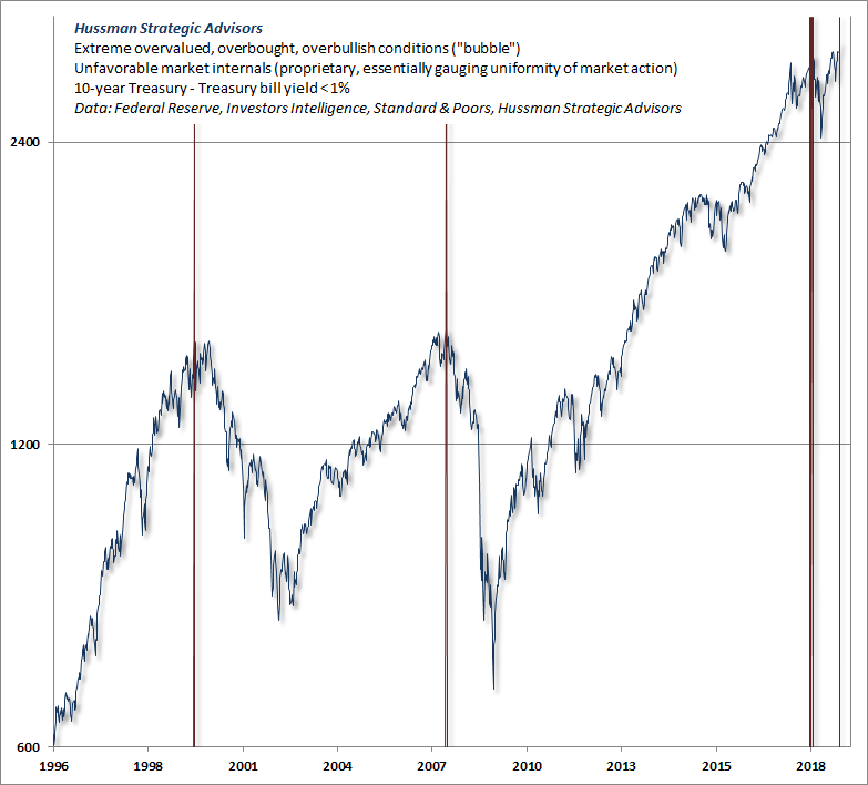
For now, we observe not only unfavorable valuations and still-divergent internals on our measures, but also the most extreme “overvalued, overbought, overbullish” syndrome we define. The only other times we’ve observed this syndrome in the context of a relatively flat yield curve (a spread of less than 1% between 10-year Treasury bond yields and 3-month Treasury bill yields) were the precise peaks of 2000, 2007, and September 2018. Narrow that spread to less than 0.5%, and only March 2000 and October 2007 remain.

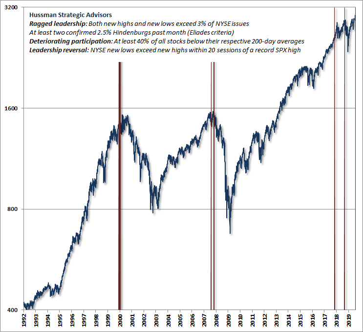
Though daily market behavior is noisy, it’s notable that in the past few weeks, the market has simultaneously registered a relatively large number of new highs and new lows among individual stocks, with a leadership reversal at the beginning of August, with new lows exceeding new highs just a week after a record high in the S&P 500. This is similar to what we observed at the 2007 market peak.

Though we don’t find much value in simplistic market indicators (e.g. some observers define a “Hindenburg” as nothing more than a single day when both new highs and new lows exceed 2.2% or 2.5% of issues traded, and these things occur all the time), broader syndromes of evidence are more informative. The accompanying chart, for example, shows the handful of instances that share the same market action we observed on Friday August 2nd, combining ragged leadership with deteriorating participation and a leadership reversal closely following a record market high.

As for last week’s rate cut by the Federal Reserve, there’s an extended discussion of Fed policy in my mid-July special market comment, but suffice it to say that the initial Fed easing following a tightening cycle has generally occurred during or immediately preceding an economic recession. Moreover, the effect of Federal Reserve policy on the stock market is highly dependent on the condition of market internals at the time.

So rather than responding directly to Fed policy, it’s important to interpret their likely effect on the markets by gauging market internals instead. As we’ve learned in the recent half-cycle, the same is has been true for “overvalued, overbought, overbullish” conditions in recent years. The condition of market internals comes first, because it directly indicates whether investors are inclined toward speculation or risk-aversion.

I’ll repeat what I’ve emphasized publicly in the past two weeks. Presently, we observe market conditions that have been associated almost exclusively, and in most cases precisely, with the most extreme bull market peaks across history. A passive investment strategy is now closer to “all risk and no reward” than at any moment in history outside of the 1929 market peak. These conditions can, of course, change. If our measures of market internals improve, we would defer an immediate bearish outlook and take a more neutral or constructive view even at these valuation extremes. Our outlook will change when the evidence changes.

The bottom line is that we have a hypervalued market, with the worst estimated prospective return for a conventional mix since the 1929 peak, divergent internals, extreme overextension, and oncoming recession risk. Whatever you’re going to do, do it.

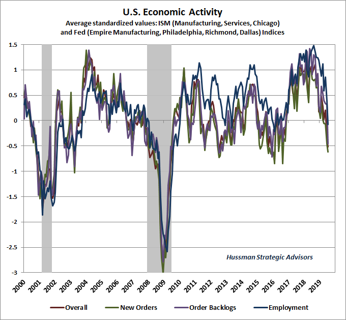
Orders and backlogs lead, production coincides, and employment lags

One of the fascinating aspects of economic discussions among Wall Street analysts and the financial media is how little consideration is typically given to ordinary leads and lags in the data. As a result, very clear economic signals are often confused using words like “cross-currents” or “mixed,” particularly around economic turning points.

The chart below shows our economic composite drawn from standardized regional and national Federal Reserve and Purchasing Managers survey data.

You’ll notice that new orders (green) have experienced the strongest plunge in recent data, with the employment line (blue) slightly lagging that decline. That’s how the sequence of economic data typically evolves. New orders and backlogs, though volatile, generally lead. Production measures, not surprisingly, tend to coincide with broad movements in economic output. Finally, employment measures lag, sometimes considerably, because decisions surrounding job creation and layoffs tend to be careful and time-consuming.

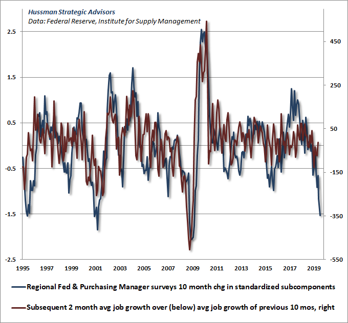
As a result, if we think in terms of a 12 month year, we find that the 10-month change in our economic activity composite tends to be well-correlated with the employment “surprise” over the next two months – defined here as the difference between the actual change in non-farm payrolls and the average change over the previous 10 months.

The collapse we’ve observed in leading economic measures over the past 10 months is now consistent with monthly job creation falling nearly -350,000 jobs short of its 10-month average of 186,000, implying potential losses of as much as -164,000 jobs per month in upcoming reports. You’ll notice in the chart below that recent non-farm payroll data has clearly bucked these progressively deteriorating expectations. The last time we saw this sort of deviation was in October 2000, a month before the U.S. economy rolled into recession. Again, employment data lags, and month-to-month data can be noisy.

It’s also important to recognize how strongly economic data tends to be revised, in hindsight, around recession turning points. For example, in the originally reported data for May through August 1990, as a new recession was emerging, the Bureau of Labor Statistics reported that 480,000 total jobs were created (see the October 1990 vintage in Archival Federal Reserve Economic Data). But in the revised data as it stands today, those figures have been revised to a loss of 71,000 jobs for the same period.

Consider early 2001. A U.S. recession had already started months earlier, but first-quarter GDP growth was initially reported at 1.2%. Based on final revision, that same quarter’s GDP growth is now reported at -1.1%. The vintage data shows that non-farm payrolls were initially reported with a gain of 105,000 jobs during January-April 2001, while the revised data now shows a loss of 247,000 jobs.

Likewise, by early 2008, the U.S. was also already in recession, but first-quarter GDP growth was initially reported at 1% growth. That figure was only later revised to -2.3%. The non-farm payroll reports were already deteriorating, with a cumulative job loss from February-May of 2008 of 248,000 jobs. Still, those initial reports pale in comparison to the revised figures, which presently show a loss of 550,000 jobs for the same period.

The collapse we’ve observed in leading economic measures over the past 10 months is now consistent with monthly job creation falling nearly -350,000 jobs short of its 10-month average of 186,000, implying potential losses of as much as -164,000 jobs per month in upcoming reports.

Given that the ISM and Fed survey data are subject to little if any revision (depending on the series), and there is a strong correlation between that data and subsequent job growth, it’s very possible that recent employment data may be revised after-the-fact. For now, we have to allow for the possibility that our present concerns will prove inaccurate, but it also seems reasonable to allow for the possibility of steep job losses ahead.

How to needlessly produce inflation

After years of extraordinary monetary policy and quantitative easing in Europe, Japan, and the United States, one thing should be clear: quantitative easing, in itself, does not produce inflation. Rather than asking why this has been so, many observers have been quick to pronounce inflation “dead,” as if the world has permanently changed, and there are no conditions that would cause inflation to bear its fangs. Advocates of “modern monetary theory” (MMT) are attracted to this idea. Others have argued that an even deeper foray into extraordinary policy is required, involving additional rounds of quantitative easing and negative interest rates. This is a popular view among central bankers.

Setting aside the rather deranged presumption that igniting inflation would somehow be durably beneficial to the economy, or that the genie, once out of the bottle, would even be controllable, we’ll focus our present discussion on the most fundamental questions: What produces inflation, and why hasn’t quantitative easing done so?

I’ve often noted that, if you spend a great deal of time with economic data, you’ll find that there is a remarkably weak relationship between inflation and variables like the money supply, or unemployment, government deficits, or the amount of slack in the economy. Somehow, we feel that these variables should be important, and we know from hyperinflations that they become important when they reach breathtaking extremes, but there’s no clear, linear relationship in the data between inflation and any of them. Indeed, the best predictor of future inflation that you’ll find in the data is the current rate of inflation.

The reason is that the value of a piece of currency, like the value of any other financial asset, depends heavily on the psychology of the holder. And psychology isn’t a nice, linear thing. Rather, just like the stock market can entirely ignore extreme valuations until investor psychology shifts from a speculative mindset to a risk-averse one (which we infer from the behavior of market internals), the tolerance of the public to hold the paper liabilities issued by the government can persist for some time, until unusually high issuance of these liabilities causes revulsion to kick in.

Then why hasn’t quantitative easing produced inflation? The answer is rather simple: quantitative easing is nothing but an asset swap. It doesn’t change the total amount of government liabilities in circulation. It only changes the form of the government liabilities that must be held by the public. The central bank buys interest-bearing government bonds, and in return it creates zero-interest base money (currency and bank reserves) that must be held instead.

QE creates a pool of zero-interest money (or when the Fed pays interest to banks on their excess reserves, low-interest money) that someone has to hold at every point in time until that base money is retired. That can certainly encourage yield-seeking speculation in financial securities, as each successive holder tries to get rid of these monetary hot potatoes. That process of speculative yield-seeking stops only when a) risky securities become so overvalued that investors become indifferent between safe, low-interest liquidity and those risky, overvalued securities, or b) investors become risk-averse enough to be happy with safe, low-interest liquidity, in which case, as investors discovered during 2000-2002 and 2007-2009, even persistent Fed easing may do nothing to stop a collapsing stock market.

What QE does not change is the total quantity of government liabilities in circulation. That decision isn’t under the control of monetary policy, but is instead determined by fiscal (tax and spending) policy.

This is a critical distinction. See, government deficits are funded by creating pieces of paper – namely government bonds, or if the central bank buys those bonds, base money. If the public believes that the government has a credible ability to retire its liabilities, or at least keep them from growing at a rate that’s not too different from the growth rate of the real economy, then people may be entirely content to hold those pieces of paper without being revolted by doing so. In that situation, the central bank can buy government bonds and replace them with base money, and vice versa, as much as it wants, and it won’t change the underlying belief that those pieces of government paper are “good” – regardless of which form they take.

Again, QE is simply an asset swap. QE doesn’t produce inflation, and whatever inflation we get will not be the result of QE. What inflation requires is public revulsion to government liabilities, and what produces public revulsion is the creation of government liabilities at a rate that destabilizes the expectation that those liabilities remain sound.

Why anyone would desire that outcome is utterly beyond me, and frankly, I’m alarmed by the entire notion of “targeting a higher inflation rate,” because my sense is that the associated revulsion would become very difficult to control. Still, if you want more inflation, the way to get it is by running government deficits that are out of line with sustainable norms. The U.S. has already placed itself on that course, but it’s not clear that we’re at the point of revulsion quite yet.

As economist Peter Bernholz has noted: “There has never occurred a hyperinflation in history which was not caused by a huge budget deficit of the state… In all cases of hyperinflation deficits amounting to more than 20 per cent of public expenditures are present.”

Moreover, even the size of the deficit has to be placed in context. See, deficits regularly expand during recessions, and tend to contract during economic expansions. The public is sufficiently familiar with this tendency that large deficits during economic downturns rarely cause inflation pressure. Rather, I would assert that revulsion generally kicks in when deficits become what I’d call “cyclically excessive” – that is, persistently larger than one would expect, given the current point in the economic cycle.

Why hasn’t quantitative easing produced inflation? The answer is rather simple: quantitative easing is nothing but an asset swap. It doesn’t change the total amount of government liabilities in circulation. It only changes the form of the government liabilities that must be held by the public.

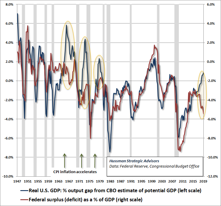
The chart below shows the U.S. real GDP output gap (the difference between actual real GDP and potential real GDP, based on Congressional Budget Office estimates), along with the U.S. federal surplus or deficit, as a percentage of GDP. Notice that the two generally move together, reflecting a tendency toward smaller deficits or even surpluses during periods of economic strength, and larger deficits during periods of economic weakness.

Notice, however, that there are a few periods when the U.S. economy was operating near full capacity (blue line near or above zero on the left scale), yet government deficits were significant and even expanding (red line well below zero on the right scale). These differences are circled in yellow. The notable feature of all of the prior instances is that they were exactly the points when the inflation rates accelerated. It’s not yet clear what will occur in the present instance, but it’s clear that the present course of government deficit spending is already significantly out-of-line with the position of the U.S. economy.

Notably, government deficits in the Euro area are also well correlated with the position of the economy within the business cycle. The primary exceptions in recent years were in 2006, when Euro area governments ran a moderate deficit despite an economy near full employment, and in 2009, when deficits were far larger than one would have expected given the level of economic slack. Not surprisingly the highest inflation rates in the Euro area during the past 20 years emerged in 2007 and 2010.

Though deficits in Japan have been substantially larger than in the U.S. or the Euro area, they also have fluctuated in sync with economic fluctuations. The main exception here occurred between 2010 and 2013, when Japanese government deficits remained far larger than one would have expected based on the accompanying level of economic slack. Again, not surprisingly, this was a period when the Japanese CPI moved from deflation to an inflation rate of 3.6% by 2013 – the highest inflation rate observed in Japan in decades.

Inflation in both Japan and Europe has undoubtedly been restrained by legal and regulatory requirements that force financial companies like insurance firms to carry large holdings of government securities. The Japanese public also has a far higher inclination to save than in most other countries. There’s no simple linear relationship even between inflation and government deficits, because institutional and psychological factors affect the willingness of the public to hold those pieces of paper.

Ironically, the revulsion to government liabilities that would be required to produce inflation has been actively prevented by regulations that are intended to allow central banks to impose negative interest rates, in the hope of producing inflation. The whole exercise is goofy.

Quantitative easing is simply an asset swap. QE doesn’t produce inflation, and whatever inflation we get will not be the result of QE. What inflation requires is public revulsion to government liabilities, and what produces public revulsion is the creation of government liabilities at a rate that destabilizes the expectation that those liabilities remain sound.

Put simply, quantitative easing merely changes the mix of securities that the public holds. Historically, inflation has been provoked by government deficits that create new government liabilities at a “cyclically excessive” and unsustainable pace. Conversely, episodes of runaway inflation have regularly been ended by restoring public faith that fiscal and monetary policy have returned to a sustainable course. In his analysis of major hyperinflations, Nobel economist Thomas Sargent (also my former dissertation advisor at Stanford) observed:

“In each case we have studied, once it became widely understood that the government would not rely on the central bank for its finances, the inflation terminated and the exchanges stabilized. We have further seen that it was not simply the increasing quantity of central bank notes that caused the hyperinflation, since in each case the note circulation continued to grow rapidly after the exchange rate and price level had been stabilized. Rather, it was the growth of fiat currency which was unbacked, or backed only by government bills, which there never was a prospect to retire through taxation.”

Again, if the public believes that the government has a credible ability to retire its liabilities, or at least keep them from growing at a rate that’s not too different from the growth rate of the real economy, then people may be entirely content to hold those pieces of paper without being revolted by doing so. Despite Milton Friedman’s dictum, inflation is not simply a monetary phenomenon. It is a fiscal one. When fiscal deficits become extreme, excessive money creation usually follows. But at its core, inflation reflects revulsion to holding government liabilities. It doesn’t actually matter whether these liabilities take the form of bonds or currency, because revulsion to those liabilities is enough to systematically devalue both of them.

In my view, the United States is already running what I’d describe as “cyclically excessive” deficits. It’s not clear yet that public revulsion has kicked in, so in the near term, economic weakness seems more likely to depress inflation and interest rates than to aggravate them. But an economic downturn would almost certainly drive U.S. government deficits to unsustainable levels, which could increase the search for alternatives to bonds and currency, adding to the upward pressure we’ve started to see in gold prices.

At present valuation extremes, the Consumer Price Index would probably need to triple before higher inflation would benefit stocks, because downward pressure on valuations would vastly outweigh the benefits of higher nominal growth rates. It’s not clear that we’re at a major inflection point for inflation yet, but it will remain important to monitor inflation-sensitive asset prices for fresh pressure on that front.

Don’t miss a market comment or special update! Join our 100% spam-free mailing list below.

---

---

The foregoing comments represent the general investment analysis and economic views of the Advisor, and are provided solely for the purpose of information, instruction and discourse.

Prospectuses for the Hussman Strategic Growth Fund, the Hussman Strategic Total Return Fund, the Hussman Strategic International Fund, and the Hussman Strategic Dividend Value Fund, as well as Fund reports and other information, are available by clicking “The Funds” menu button from any page of this website.

Estimates of prospective return and risk for equities, bonds, and other financial markets are forward-looking statements based the analysis and reasonable beliefs of Hussman Strategic Advisors. They are not a guarantee of future performance, and are not indicative of the prospective returns of any of the Hussman Funds. Actual returns may differ substantially from the estimates provided. Estimates of prospective long-term returns for the S&P 500 reflect our standard valuation methodology, focusing on the relationship between current market prices and earnings, dividends and other fundamentals, adjusted for variability over the economic cycle.