How to Spot a Bubble

 

John P. Hussman, Ph.D.
President, Hussman Investment Trust

March 2021

---

I can show, really precisely, that there are two warranted prices for a share. The one I prefer is based on such fundamentals as earnings and growth rates, but the bubble is rational in a certain sense. The expectation of growth produces the growth, which confirms the expectation; people will buy it because it went up. But once you are convinced that it is not growing anymore, nobody wants to hold a stock because it is overvalued. Everybody wants to get out and it collapses, beyond the fundamentals.

– Nobel Laureate Franco Modigliani, New York Times, March 30, 2000

The word “bubble” is tossed around quite a bit in the financial markets, but it’s rarely used correctly. See, the thing that defines a bubble isn’t that valuations are extremely high, or that expected returns are extremely low. Instead, what defines a bubble is that investors drive valuations higher without simultaneously adjusting expectations for returns lower. That is, investors extrapolate past returns based on price behavior, even though those expectations are inconsistent with the returns that would equate price with discounted cash flows.

In March 2000, at the height of the technology bubble, I noted: “Over time, price/revenue ratios come back in line. Currently, that would imply an 83% plunge in tech stocks. If you understand values and market history, you know we’re not joking.” The following month, I discussed Modigliani’s quote above, and detailed the dynamics he was describing. The collapse of the 2000 bubble would ultimately erase half the value of the S&P 500, and would take the tech-heavy Nasdaq 100 down an implausibly precise 83%.

The defining feature of a bubble is inconsistency between expected returns based on price behavior and expected returns based on valuations. If investors pay $150 today for a security that will deliver a single $100 payment a decade from now, but they also fully understand that they’ll lose 4% annually on the deal, without extrapolating past gains into the future, then we might say the security is overvalued, and we might question why investors would accept that trade, but we can’t call it a bubble.

But if investors pay $150 today for that security, because they look back in the rear-view mirror, decide that it “always goes up” over time, and convince themselves that expected future returns are always positive, then you’ve got a bubble. Discounting the future $100 cash flow of the security using any positive expected return would produce a price less than $100. So the positive returns expected by investors are inconsistent with the returns that would equate price with discounted cash flows. The size of the bubble is the fraction of the market price that represents expectational “hot air.”

Likewise, the willingness of investors to embrace “passive investments” like ETFs and asset-backed securities based on past performance, with little concern about the valuations, yields, or credit risk of the securities inside, is a the very soap from which bubbles repeatedly emerge. Amid the current enthusiasm for special purpose acquisition companies (SPACS), investors might recall the bubble in “incubators” at the 2000 peak, the “conglomerates” of the late-1960’s Go-Go bubble, and even the South Sea Company in the early 1700’s, along with similar companies formed at the time “for carrying on an undertaking of great advantage, but nobody to know what it is.”

If investors price the S&P 500 at levels that are highly likely to produce negative returns for a decade, as they did in 1929 and 2000, and as I believe they are doing at present, yet investors continue to press stock prices higher on the expectation that they will provide historically normal levels of future return regardless of valuations, then you have the sort of inconsistency that defines a bubble.

Likewise, if the expected return of a conventional passive investment mix is negative on a 10-12 year horizon (based on reliable valuation measures strongly correlated with actual subsequent returns over a century of market history), yet pension return assumptions remain locked near 7% annually, you’ve got a bubble, and most likely a future pension funding crisis, on your hands.

This is how very bad things have repeatedly happened in the financial markets across history, enabled by what Galbraith called “the extreme brevity of the financial memory.”

When Modigliani says that there are two “warranted” prices, he means that – at least in the short run – there are two ways that prices can fulfil the expectations of investors. In one case, investors have expectations about future returns, and those expectations are informed by the level of valuations. If prices rise, and expected cash flows haven’t changed, investors recognize that future returns will be lower. In the “bubble” case, investors have high expectations about future returns, mainly based on past returns, and they act on those expectations by driving prices up further. So the expectation of additional price increases is simply reinforced. “The expectation of growth produces the growth, which confirms the expectation.”

Only one of these prices is consistent, in that the rate of return expected by investors is also the rate of return that equates price with discounted future cash flows. The other price becomes increasingly detached from fundamentals, as a larger and larger fraction of the price represents hot air, and it ultimately collapses as the gap becomes untenably wide.

What defines a bubble is that investors drive valuations higher without simultaneously adjusting expectations for returns lower. That is, investors extrapolate past returns based on price behavior, even though those expectations are inconsistent with the returns that would equate price with discounted cash flows. The defining feature of a bubble is inconsistency between expected returns based on price behavior and expected returns based on valuations.

During speculative segments of the market cycle, there’s nothing that forces investors to recognize that higher valuations imply lower returns, or to change their expectation of high returns as far as the eye can see. That, of course, is why we use measures of market internals to gauge the inclination of investors toward speculation or risk-aversion. Valuation provides an enormous amount of information about likely long-term returns and potential market losses over the complete cycle. But valuation isn’t a timing tool. In recent years, it hasn’t even imposed a limit on speculative recklessness.

Still, with each price advance, the actual long-term return implied by future cash flows – what investors will ultimately realize as those cash flows are delivered – collapses further, even while investors act on their delusion that long-term returns have nothing to do with price. Eventually, the bulk of the security price represents a bubble component, not the price that would actually need to exist in order for the long-term expectations of investors to be accurate.

As I wrote at the 2000 market peak:

“As long as investors focus on year-to-year returns and not discounted cash flow calculations, the bubble can continue to grow in self-reinforcing fashion. Investors anticipate a high return, and the price behavior reinforces the expectation. The true long-term return becomes increasingly detached from the long-term return imagined by investors, and the bubble component accounts for an increasingly large proportion of the total price.”

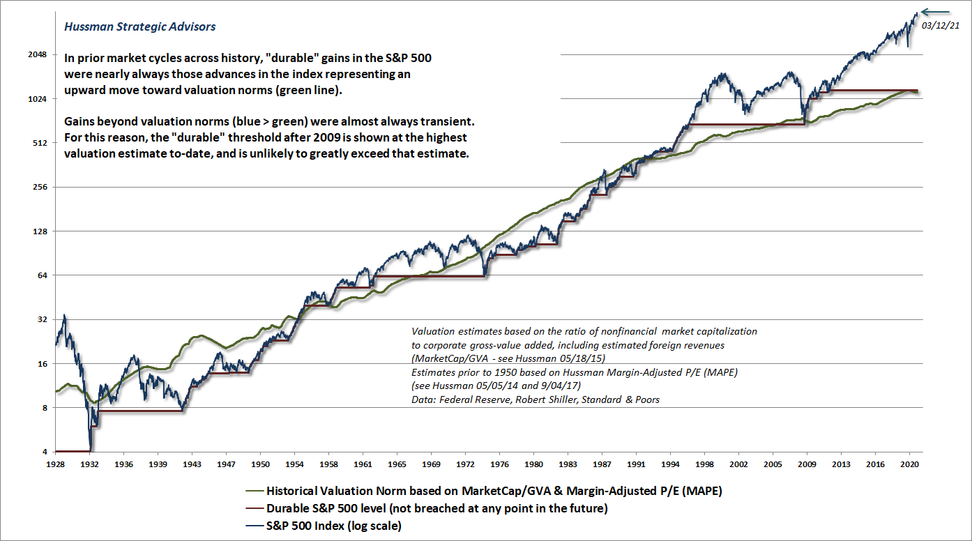
By our most reliable measures, run-of-the-mill historical valuation norms are roughly 70% below current levels. I know you don’t want to believe that.

The trap door quietly swings open when valuations are extreme and market internals begin to deteriorate. That’s the situation we’ve observed in our measures in recent weeks, with the initial deterioration largely driven by debt securities, but with increasing divergences in equities as well.

Valuations and discounted cash flows

Valuations measure the tradeoff between current prices and a very long-term stream of expected future cash flows. Every useful valuation ratio is just shorthand for that calculation. Every valuation ratio that fails that criterion is inferior, and you can show it in historical data.
– John P. Hussman, Ph.D., The Meaning of Valuation, December 2019

I’ve often noted that the denominator of every good valuation measure is just shorthand for the decades and decades of cash flows that the security is likely to deliver in the future. In fact, we always test the validity of the valuation measures we use by examining:
a) how strongly the resulting valuation measures are correlated with actual subsequent total returns, and;
b) how closely they replicate an explicit discounted cash flow analysis.

Below, we’ll examine a variety of valuation measures that offer some perspective on why I view the U.S. equity market as a bubble near the breaking point. Along the way, I’ll point out some interesting features of valuations and their relationship with subsequent returns. If math gives you hives, feel free to skim over the small amount that I’ve included here and there.

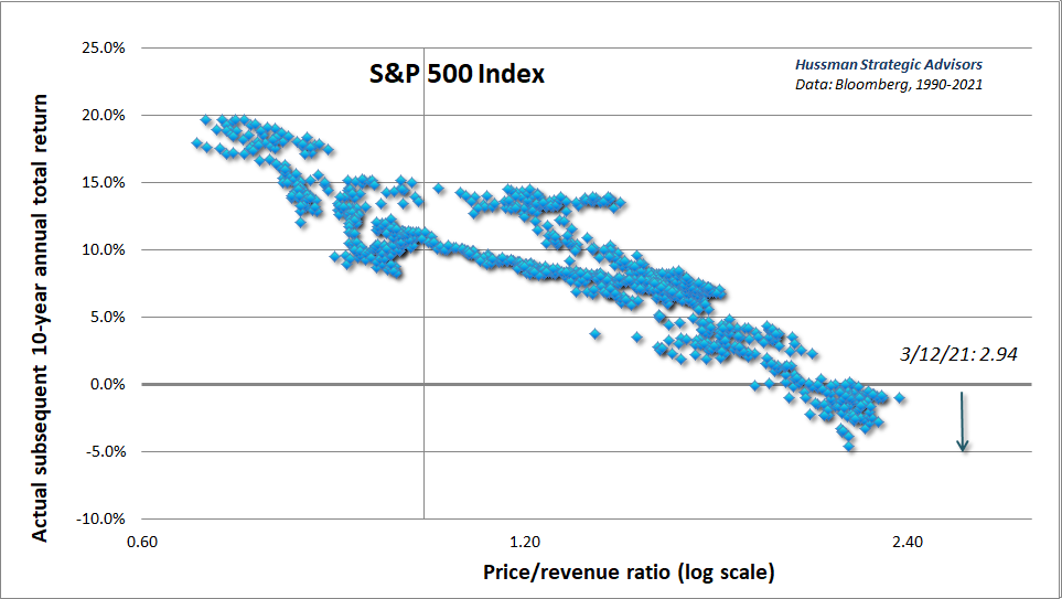
Consider first the relationship between valuations and subsequent returns. I’ll state the following, which you can prove to yourself by toying around a bit with present value models: the logarithm of a good valuation measure should have an inverse and roughly linear relationship with the expected subsequent investment return.

Here’s a simple example of what this looks like.

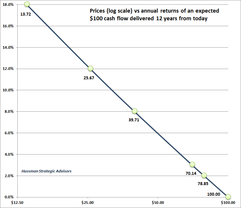
The logarithm of a good valuation measure should have an inverse and roughly linear relationship with the expected subsequent investment return.

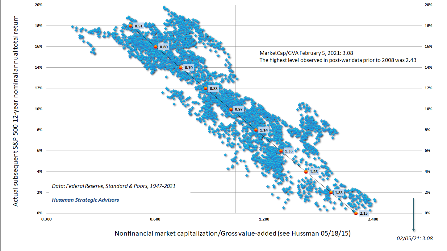
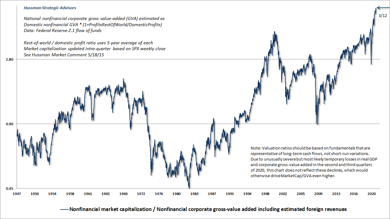
Here’s what this looks like for MarketCap/GVA, our most reliable stock market valuation measure

During the past three decades, we’ve studied and introduced a broad range of valuation measures. Most can be calculated back to 1947. Some can be evaluated over a century or more. Across history, even in recent decades, we find that the valuation measures that are best correlated with actual subsequent returns are those with muted sensitivity to cyclical fluctuations in profit margins, and that behave largely like broad, market-wide price/revenue ratios.

The denominator of every good valuation measure is just shorthand for the decades and decades of cash flows that the security is likely to deliver in the future.

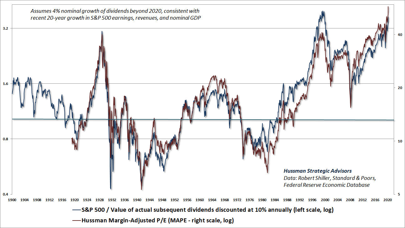
If we compare our most reliable valuation measures with the valuation measures that one would obtain from a proper long-term discounted cash flow analysis, we find that they’re nearly identical. Here’s what this comparison looks like for the actual stream of dividends (including impact of repurchases) delivered by the S&P 500 since 1900, discounted at a fixed 10% rate (see the chart text for additional details). The reason we use a fixed rate of return is that a multiple of 1.0 is then, by definition, the level at which the S&P 500 would have been priced for that particular level of expected return. Any deviation in the valuation multiple from 1.0 then gauges how far likely future returns are from that “typical” expected return. We’re currently farther away from “typical” expected returns than at any moment in history, including the 1929 and 2000 market peaks.

One of the unfortunate bits of financial illiteracy that Wall Street has pushed into the heads of investors is the idea that extreme valuations are “justified” by low interest rates. Now, it’s certainly true that, holding future cash flows constant, raising the price of an investment will lower the embedded rate of return, and vice versa. If you pay $32 today for $100 a decade from today, you can expect a 12% annual return. If you pay $82 for the same security, you can expect a 2% annual return. If you pay $100 today, you can expect nothing. So it’s clearly true that, holding future cash flows constant, a lower rate of return implies a higher level of valuation.

The reason the statement “low interest rates justify high valuations” contributes to financial illiteracy is that the statement has been learned entirely out of context of the arithmetic. As a result, investors seem to imagine that, as long as high valuations can be “justified,” stocks can be expected to provide historically normal rates of return in the future. Likewise, investors seem to have no concept that if interest rates are low because growth rates are low, no valuation premium is “justified” for stocks, because the lower growth is already sufficient to bring future stock returns down to levels that are commensurate with the low level of interest rates.

The truth is simple but uncomfortable. If interest rates are low and expected growth is held constant, higher valuations imply lower long-term returns. If interest rates are low because expected future growth is also low, higher valuations are not required. Long-term returns will be lower anyway. A valuation premium just makes future returns even worse.

Saying that extremely low interest rates “justify” extremely high stock valuations is identical to saying that extremely low future returns on bonds “justify” extremely low future returns on stocks. I don’t really think that’s something Wall Street cares to clarify when it tells investors that stock market valuations are “justified.”

Investment valuation is concerned with the relationship between three objects: the current price, the future cash flows, and the rate of return that connects the two like a string. The lower the current price and the higher the future cash flows, the steeper the string. The higher the current price and the lower the future cash flows, the flatter the string. Raise the current price above the future cash flows, and the string will point down instead of up. Given any two of these objects, you can calculate the third one.

For example, if you want to estimate expected long-term returns, you need two objects: a) the current price and b) the expected stream of future cash flows. A good valuation ratio is just shorthand for those two objects, so you can estimate the long-term return directly from the level of valuation. Then, if you like, you can compare it with the level of interest rates. That comparison can be useful, because even when investors realize that high stock market valuations imply low long-term returns, it’s not at all clear that they realize how low long-term return prospects have been driven.

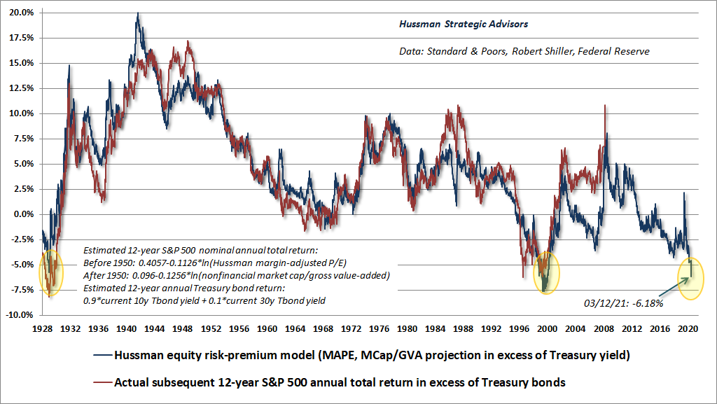
The chart below shows our estimate of expected 12-year S&P 500 total returns over-and-above Treasury bond yields, across a century of market history. Compare this with the nearly useless drivel that Wall Street passes off as the “equity risk premium” (typically quoted as the S&P 500 forward earnings yield minus the 10-year Treasury yield). Yes, you’re reading the chart correctly. Given current valuations, we expect the total return of the S&P 500 to underperform the lowly yield on Treasury bonds by roughly -6% annually over the coming 12-year period.

Many investors confuse the estimation of expected returns (which requires only expected cash flows and the observed price) with a different problem – the estimation of “fair value.” See, interest rates come into the picture when you have an expected stream of future cash flows and you want calculate a “fair” current price. In that case, rather than picking an arbitrary rate of return from a hat, it’s common to use the level of interest rates, plus some risk premium, as the expected long-term return (or discount rate, or capitalization rate). This sort of calculation can be super-sensitive to arbitrary choices. In particular, Wall Street loves to combine super-high growth rates, super-low discount rates, and super-long time horizons, which allows one to calculate a “fair value” that’s as close to infinity as possible. The thing to remember is that whatever rate of return an analyst embeds into the fair value calculation is also the long-term rate of return you’ll earn over time if you pay that price, assuming the future cash flows are delivered as expected.

The truth is simple but uncomfortable. If interest rates are low and expected growth is held constant, higher valuations imply lower long-term returns. If interest rates are low because expected future growth is also low, higher valuations are not required. Long-term returns will be lower anyway. A valuation premium just makes future returns even worse.

Among scores of measures we’ve evaluated or introduced over time, MarketCap/GVA (nonfinancial market capitalization to corporate gross value-added, including our estimate of foreign revenues) has the highest correlation with actual subsequent 10-12 year S&P 500 total returns, followed by our Margin-Adjusted P/E (MAPE). I find it hilarious that the various valuation measures I’ve introduced over time are sometimes described as products of “machine learning,” “data mining,” and “curve fitting” when they are, in fact, just different versions of an apples-to-apples economy-wide price/revenue ratio.

The S&P 500 price/revenue ratio and nonfinancial market capitalization to GDP (the “Buffett indicator”) also perform well, and better than earnings-based alternatives like price/forward earnings, the Fed Model, and even the Shiller CAPE. See, while earnings are necessary to generate long-term cash flows, they are also subject to fluctuations in profit margins (both cyclically and even from decade to decade) that turn out to be highly uninformative.

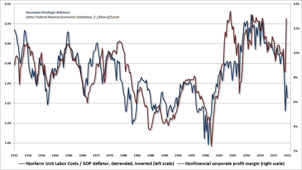
Economically, fluctuations in profit margins are driven primarily by fluctuations in real unit labor costs. Because companies compete on the basis of realized after-tax profits rather than pre-tax profits, changes in tax policy also have far less durable impact on corporate profits than investors seem to imagine. While corporate profits got a tremendous boost last year from CARES spending (the deficit of one sector always emerges as the surplus of another), here’s what the relationship between corporate profits and real unit labor costs looks like historically. Real unit labor costs are presented on an inverted left scale. The upward pressure on labor costs (observed as a plunge in the blue line) isn’t particularly auspicious for future profits. Still, there’s so much distortion in recent quarters that I’d consider the jury to be out on how much of this will be sustained.

It’s undoubtedly true that profit margins, expected growth, and other factors have an effect on future deliverable cash flows and the valuations that investors place on stocks. But even for technology stocks, these assumptions should be made explicit and tested against history. You’ll find that observable measures like price/revenue are still very serviceable. In fact, the extreme price/revenue multiples of technology stocks helped to inform my March 2000 projection of an 83% loss in that sector.

As Benjamin Graham wrote, “The habit of relating what is paid to what is being offered is an invaluable trait in investment. The more dependent the valuation becomes on anticipations of the future – and the less it is tied to a figure demonstrated by past performance – the more vulnerable it becomes to possible miscalculation and serious error.”

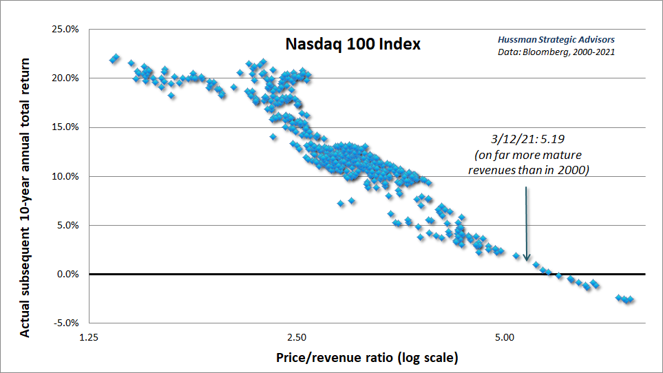
The current 5.19 price/revenue multiple for the Nasdaq 100, is the most extreme level since February 2001, which was followed by a 60% loss in the index (after it had already dropped in half). The situation is actually a bit worse than 2001 here. If one examines the largest components of the index, it becomes clear that their annual growth rates have declined substantially over time. As a result, a dollar of current revenues should arguably command a smaller multiple than a dollar of revenues might have during earlier periods of emerging growth. Yet even if one takes the Nasdaq 100 price/revenue ratio at face value, and even if one restricts attention to the bubble period since 2000, it’s difficult to expect the Nasdaq to produce total returns over the coming decade much better than zero.

You don’t really want to see what the same chart looks like for the S&P 500.

The same is true, unfortunately, for passive investment strategies. We presently estimate negative 12-year average annual total returns for a conventional passive investment mix invested 60% in the S&P 500, 30% in Treasury bonds, and 10% in Treasury bills.

In a 2019 white paper, I detailed an approach to estimate a “value-focused asset allocation” by jointly considering prevailing stock market valuations and interest rates. It specifies an investment allocation based on which asset class is estimated to have the highest average annual expected return, adjusted for risk, to each point in a long-term investment horizon. That allocation can then be modified by a risk-management component, to adjust exposure during segments of the market cycle where risk-aversion or speculation among market participants may temporarily drive valuations to depressed or elevated levels. The white paper includes numerous charts showing how this value-focused asset allocation has changed across market history, particularly at important peaks and troughs in the stock and bond markets.

Along with those methods, I introduced our “Endowment/spending multiple,” which estimates the number of years of spending that a passive 60/30/10 investor requires up-front, in order to finance an expected 36-year stream of future inflation-adjusted spending. The idea here is that in a deeply undervalued market with high expected future returns, investors can finance a future stream of spending with far less than they require when valuations are extreme and prospective returns are low.

You know you’re in a bubble when funding a 36-year stream of expected inflation-adjusted spending requires over 38 years of money up-front.

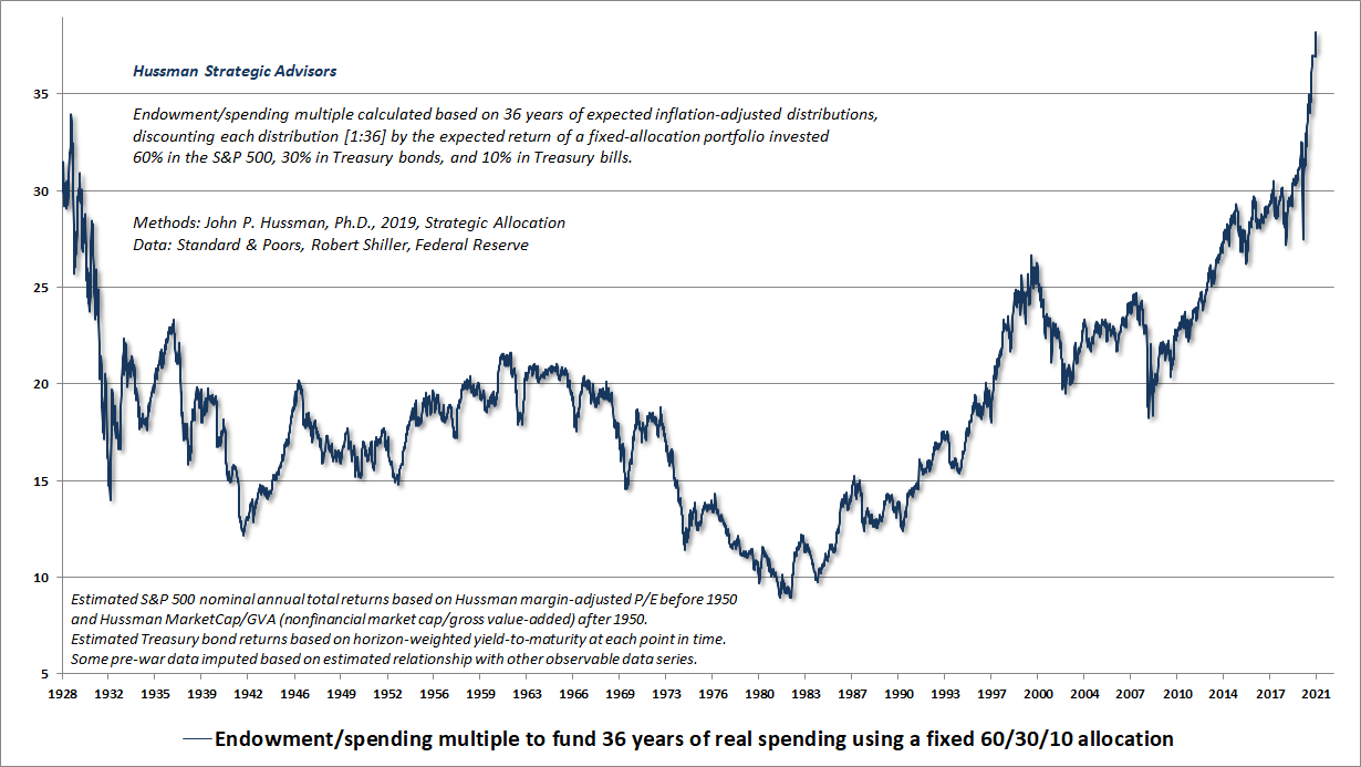
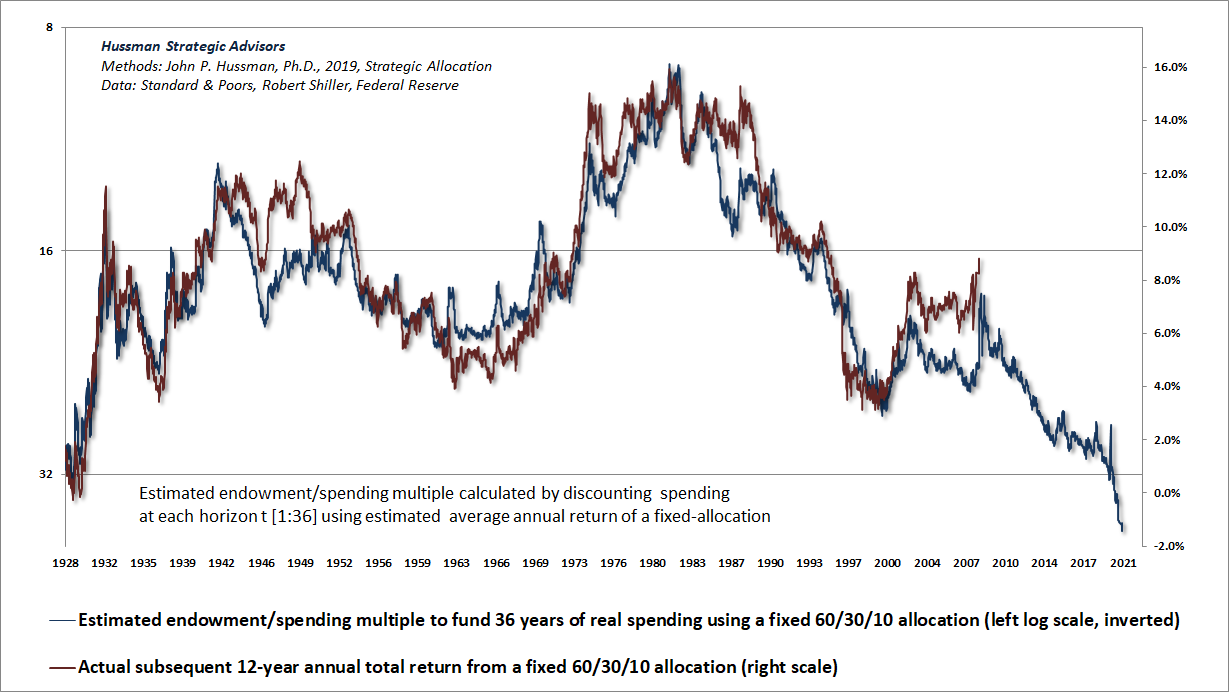
In the chart below, the Endowment/spending multiple is presented on an inverted log scale (left), along with the actual subsequent average annual total return of a 60/30/10 portfolio mix (right scale). Needless to say, we adhere to investment disciplines that are intended to address problems like this.

You know you’re in a bubble when funding a 36-year stream of expected inflation-adjusted spending requires over 38 years of money up-front.

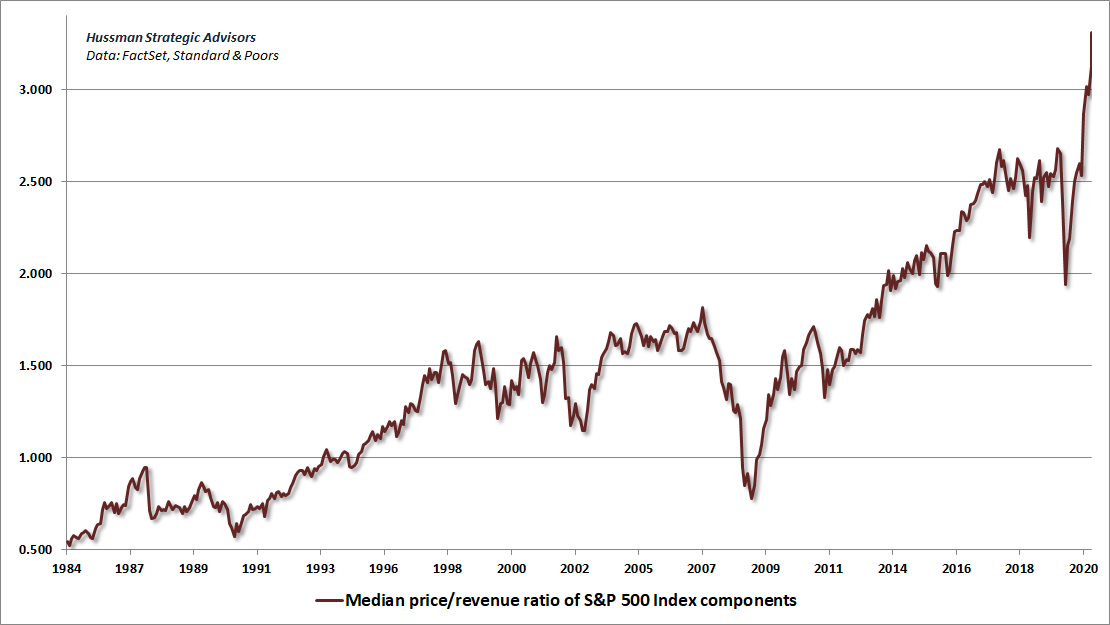
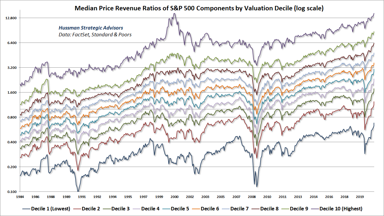
As a testament to the breadth of this speculative episode, the median price/revenue ratio of S&P 500 components now exceeds 3.3, easily a record, and extreme enough to provoke distress about the potential losses that innocent but poorly-informed investors may experience over the completion of this cycle.

The next chart shows the median price/revenue ratio of S&P 500 components sorted into 10 deciles by valuation. The chart is presented on log scale to allow each line to be compared with its own history. Each segment on the vertical axis represents a doubling of valuations. Notice that every single decile of S&P 500 components is at record valuation extremes. Investors now rely on a permanently high plateau in these extremes.

It’s interesting, but far less important, that the median price/earnings ratio of S&P 500 components has also reached 32.4, the highest level in history. This compares with a median P/E of 19.4 at the 2000 market peak. The problem with P/E multiples, of course, is that they are substantially affected by earnings variability. In fact, prior to the current peak, the highest median P/E for the S&P 500 was actually in March 2002, when the index was down 25% from the March 2000 bubble highs. That’s because earnings were down far more by then, which boosted P/E ratios. Such is the danger of taking P/E multiples at face value.

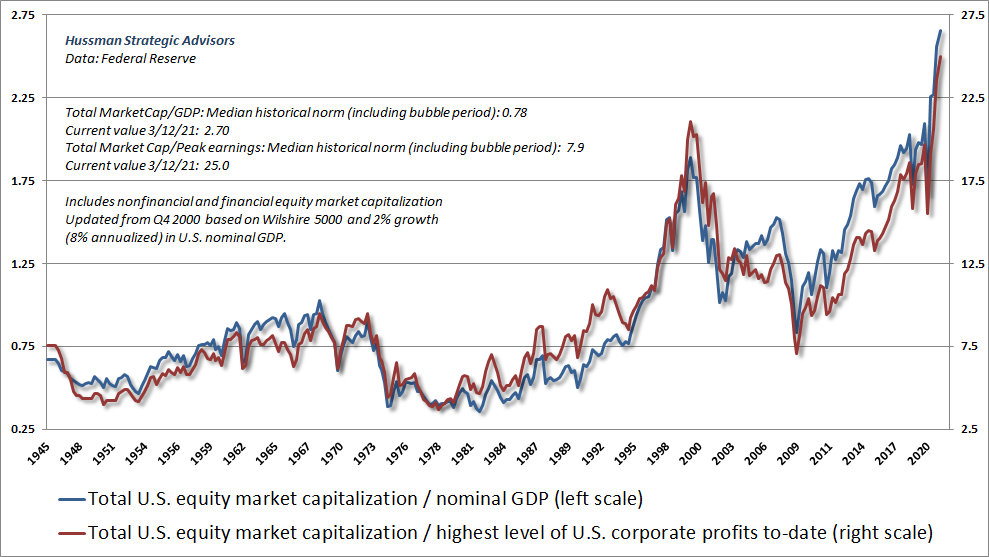
A crude but reasonably effective way to get around the cyclicality of earnings (but only for very broad indices), is to compare prices to the highest level of earnings achieved to-date. I introduced this metric back in 1998 as the price-to-peak-earnings ratio. The chart below shows a version of that. The blue line (left scale) shows the ratio of total U.S. equity market capitalization to GDP. The red line (right scale) shows the ratio of total U.S. equity market capitalization to the highest level of economy-wide U.S. profits to date. Investors have gotten themselves into trouble here.

What if valuations remain extreme forever?

Probably the single most frequent question I’ve heard from investors over the past couple of years is “What happens if valuations remain extreme forever?” It’s actually a version of the “permanently high plateau” that Irving Fisher disastrously projected in 1929. Still, recent years have produced enormous confidence among investors that the Federal Reserve’s purchases of Treasury debt can permanently “backstop” the stock market.

As I’ve detailed previously, quantitative easing supports the market only by creating zero interest hot potatoes that are uncomfortable for investors to hold (provided that they’re inclined toward speculation), and that are impossible to get rid of in aggregate. Moreover, the Fed’s purchases of corporate bonds during the pandemic were legally constrained to CARES funds provided by the Treasury, and ultimately amounted to $14 billion of bonds, in an economy with $11 trillion in corporate debt at $58 trillion in equity market capitalization.

Suffice it to say that the “Fed backstop” is largely in the minds of investors, and relies almost exclusively on the psychological discomfort of holding low-yielding base money. Yet since perception can be indistinguishable from reality, particularly in the short run, it’s important to entertain the question.

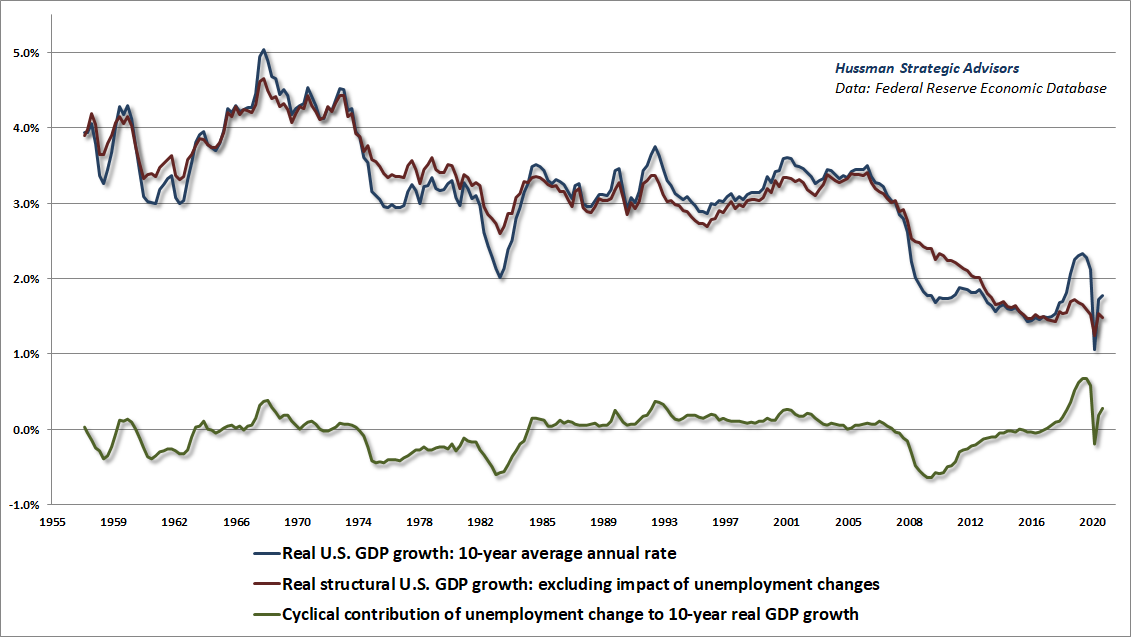
My answer is that if the Fed is indeed able to maintain valuations at the highest levels in history, forever, stock prices would likely grow at roughly the same rate as nominal GDP. So figure 1.6% real structural growth plus 2% inflation gets you 3.6%. Let’s call it 4%, which would match nominal GDP growth in both the 10-year and 20-year periods ending at the Q4 2019 economic peak, just before the pandemic. The first casualty of rising inflation is stock valuations, so it’s not at all clear that assuming higher inflation would help stocks until valuations were roughly normalized, which would require consumer prices to roughly triple.

The chart below is a reminder of how structural real GDP growth has progressed over recent decades (driven by demographic labor force growth and trend productivity), and the basis for that 1.6% figure for structural real GDP growth.

Sticking with 4% nominal growth, and adding a 1.5% dividend yield, a “permanently high plateau” in market valuations would imply S&P 500 total returns of about 5.5% annually. Again, this assumes that valuations never retreat from levels that presently stand at about 3.6 times their historical norms. Simply allow them to retreat to 2.4 times their historical norms a decade from now – which would still keep valuations among the highest 10% in U.S. history – and the resulting 10-year total return would drop to about 1.3%. I think this would actually be the best-case scenario even in a permanently overvalued world.

At elevated valuations, even very small changes in expected return imply enormous changes in prices. So it’s unlikely that a period of much higher average valuations will escape the prospect of relatively high volatility. Rather than a 70% market decline, which would presently be required for the S&P 500 to simply touch historically run-of-the-mill valuation norms, investors could expect rather frequent market losses in the 20-35% range, which is essentially what we’ve seen even over the past few years.

All of that would be fine with us. We’ve adapted our discipline sufficiently (especially in late-2017) to tolerate the possibility of permanently sustained overvaluation. My impression is that the impact of those adaptations has become more evident as we’ve had greater opportunities to live into them. I can’t say that I believe for a second that investors will actually be spared from a 50-70% loss in the S&P 500 in the coming years, but again, it will be fine with us if the market never approaches historical valuation norms again. With the adaptations we introduced in late-2017, our discipline is flexible enough to navigate a bubble even without embracing its premise.

An unusual overlap of high-risk conditions

Returning to Modigliani, my impression is that the advance of recent years to the most extreme valuations in history reflects exactly the bubble dynamics he described, and I expect that it will also end as he described (though not necessarily in one fell swoop): “The expectation of growth produces the growth, which confirms the expectation; people will buy it because it went up. But once you are convinced that it is not growing anymore, nobody wants to hold a stock because it is overvalued. Everybody wants to get out and it collapses, beyond the fundamentals.”

One of our internal gauges tracks the correlation of market conditions with certain high-risk features that have preceded steep market collapses – a collection of measures capturing valuations, internals, sentiment, leverage, overextension, and yield pressures. Only a handful of instances in history overlap pre-crash conditions as well as they do at present. The current overlap is actually quite similar to August 1987. Meanwhile, the correlation of current conditions with features typically observed at market lows is the most negative in history.

If you want my opinion, I suspect that a near-vertical market plunge on the order of 25-35% is coming, probably quite shortly, most likely out of the blue, as in 1987, driven by nothing more than the sudden concerted effort of overextended investors to sell, and the need for a large price adjustment in order to induce scarce buyers to take the other side.

As usual, no forecasts are necessary. We’ll align our investment stance in response to the valuations and market action that we observe at each point in time. Still, it’s of particular concern that these overlaps are occurring in the context of the most extreme valuations in history, along with strikingly dysfunctional pockets of illiquidity in many individual issues. This dysfunctional behavior isn’t about any particular video game retailer. I suspect it’s actually about some sort of fragility or segmentation in order-flow mechanisms, possibly coupled with poorly managed derivatives exposure.

As I used to teach my students, show me a financial debacle, and I’ll show you someone who had a leveraged, mismatched position that they were suddenly forced to close into an illiquid market.

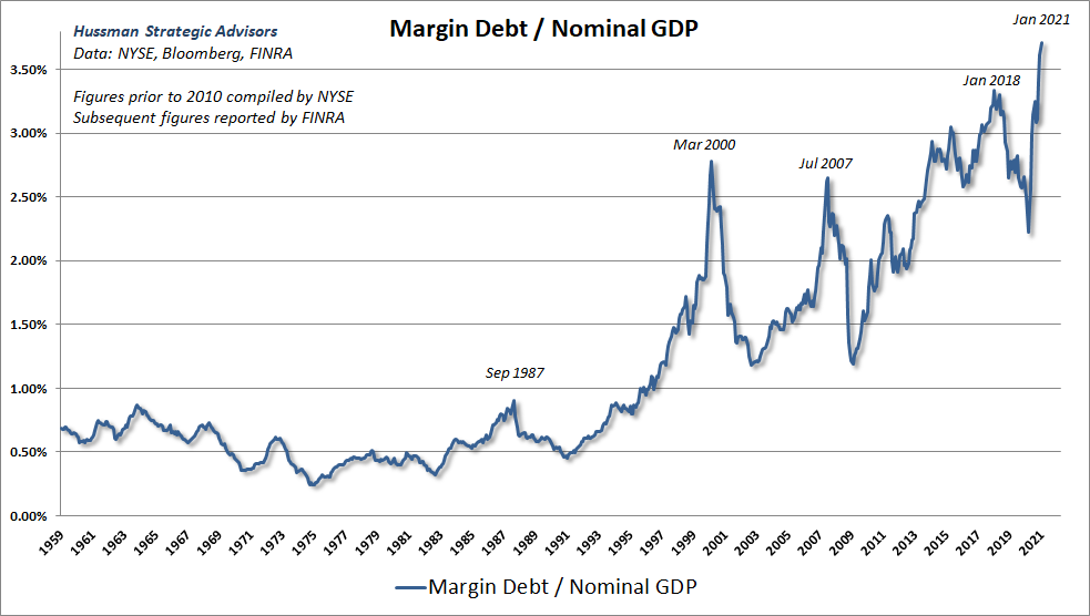
Though my concerns run far beyond the amount of leverage in the system, it isn’t helpful that the amount of leverage in the U.S. equity markets is now easily the highest in history. Some observers are inclined to bring this figure down by dividing instead by the market capitalization of equities. But here’s some useful arithmetic:

Margin Debt/GDP = Margin Debt/Market Cap x Market Cap/GDP

To say that margin debt to GDP is at the highest level in history is to say not only that stocks are heavily owned on margin, but that those stocks are also breathtakingly overvalued. That combination is particularly worrisome.

All crises have involved debt that, in one fashion or another, has become dangerously out of scale in relation to the underlying means of payment.
– John Kenneth Galbraith, A Short History of Financial Euphoria

The kind of event I’m suggesting would not bring valuations anywhere near historical valuation norms. Given current valuation extremes, it would be more like a palate cleanser. I have no particular expectation about what the next dish would be. In the event we do observe an abrupt market collapse, the Fed will undoubtedly respond with some new palliative. Whether or not it is effective will depend on the context of risk-aversion, inflation, credit risk, and other conditions at the time. The larger problem, as we’ve discussed, is that you can’t “save” an overvalued asset by propping up its price. The value is in the future cash flows that will be delivered to investors over time. The elevated price only ensures that the long-term return between now and then will be dismal.

Of course, nothing in our discipline relies on a market plunge. Given the combination of hypervaluation and divergent market internals (largely based on debt securities, but with increasing divergences in equities as well), I do believe that the stock market remains in a “trap door” situation. Still, that view will change as market conditions change. We’ll refrain from adopting or amplifying a negative outlook if our measures of market internals improve. That discipline has served us well even amid record highs. Again, no forecasts are required, nor does this opinion drive our current investment stance. I just think the correlation with historical pre-crash conditions is worth noting.

How little, it will perhaps be agreed, was either original or otherwise remarkable about this history. Prices driven up on the expectation that they would go up, the expectation realized by the resulting purchases. Then the inevitable reversal of these expectations because of some seemingly damaging event or development or perhaps merely because the supply of intellectually vulnerable buyers was exhausted. Whatever the reason (and it is unimportant), the absolute certainty is that this world ends not with a whimper but with a bang. And so on to the moment of mass disillusion and the crash. This last, it will now be sufficiently evident, never comes gently. It is always accompanied by a desperate and largely unsuccessful effort to get out.
– John Kenneth Galbraith on the 1929 collapse

Valuations and investment duration

To understand why extreme valuations imply high volatility, and require extremely long investment horizons, it’s useful to consider the concept of “duration.”

Every security is a claim on a stream of future cash flows that can be expected to be delivered to the investor over time. While the concept of “duration” is most commonly used for bonds, it’s actually applicable to any security, no matter how “lumpy” the stream of cash flows might be.

If you don’t like math, feel free to skim over the various equations and just read the pull quotes. I’ve provided the details just for completeness.

The “duration” of a security can be defined in two ways.

Investment horizon: the weighted average number of years it takes for the security to deliver its payments. For each period, you take the share of total present value represented by that year’s payment, and multiply it by the number of years in the future the payment will be received. Add them all up. The result is number of years from today (a weighted average) that the present value of your investment will be repaid. For example, the duration of a security that delivers a single payment a decade from now is simply 10 years.

Elasticity: the percentage change in the security in response to a change in the underlying gross rate of return. Technically, elasticity is (-dP/P)/(dk/1+k). For example, suppose you own a security that will pay $100 a decade from now, and it’s priced at $82.0348, for a 2% annual return. Now assume the expected return moves to 2.01%. The price would drop to $81.9544. Elasticity is (0.0804/82.0348)/(0.0001/1.02) = 10%

It turns out that the “duration” of a security in years is identical to its “duration” in terms of the percentage change of price in response to a 1% fluctuation in expected returns. Duration is also the holding period that “immunizes” the investor against changes in expected returns over time. In other words, assuming you reinvest your cash flows over time, duration gives you a good idea of how long you have to hold the security in order for your ending wealth to be largely independent of the fluctuations that the security experiences over that horizon.

Historically, investors wishing to match the duration of their investment portfolio to the duration of their investment horizon could be reasonably comfortable holding 100% of their assets in stocks, provided they had an investment horizon of about 25-30 years. Presently, these investors would need an investment horizon closer to 65-70 years. They are currently holding sippy cups.

If you know differentiation, can prove to yourself that the “modified duration” of the S&P 500 is essentially the inverse of the dividend yield. The modified duration is just (-dP/P)/dk or Macaulay duration/(1+k).

Consider P = D/(k-g). Differentiating with respect to k, dP/dk = -P/(k-g), so duration (-dP/P)/dk = P/D.

Here’s how to think about the link between valuations and duration. Presently, the dividend yield of the S&P 500 is 1.48%. If the yield moves to 1.49%, holding dividends constant, prices drop by 1.48/1.49-1 = -0.67% on that 1 basis point move. Duration is just that sensitivity, defined for a 100 basis point move, which would be 67. It turns out that’s also the weighted-average number of years from today that you’ll receive your present value, if you invest today.

Compare that to the typical situation over the past century, when the dividend yield of the S&P 500 averaged about 3.7%. At normal valuations, a 1 basis point increase in the dividend yield would produce a price drop of 3.7/3.71-1 = 0.27%, implying a duration of 27 years.

It turns out that the ‘duration’ of a security in years is identical to its ‘duration’ in terms of the percentage change of price in response to a 1% fluctuation in expected returns. Duration is also the holding period that ‘immunizes’ the investor against changes in expected returns over time.

Historically, investors wishing to match the duration of their investment portfolio to the duration of their investment horizon could be reasonably comfortable holding 100% of their assets in stocks, provided they had an investment horizon of about 25-30 years. Presently, these investors would need an investment horizon closer to 65-70 years. They are currently holding sippy cups.

Scarcity, usefulness, and value

While we’re on the subject of bubbles, I’ll add a few comments on Bitcoin, just for fun. I’d write more, but my sides still hurt from laughing.

Objects like tulip bulbs and Bitcoin differ from securities in that they do not deliver a stream of cash flows to the holder. Instead, what objects like tulips and currencies provide is a little stream of services over time, for example, as a perennial thing of beauty or as a means of payment. What people sometimes forget is that it is not just scarcity that defines the value of an object, but the stream of useful “services” that it provides (for some reason, nobody wants to buy my unique, limited edition, digitally-signed porcupine seat covers). The price of the object, and the stream of services it provides, should be commensurate.

U.S. dollars, for example, have value primarily because they are tethered to the real economy by fiat (they legally must be accepted as a means of payment, as noted on the face of any dollar bill), and they represent the entire substrate of the banking system – nearly every payment that goes back and forth in the U.S. economy represents a transfer of base money. Base money (currency and bank reserves) provides billions of little “services” over time. With every transaction, reserves move electronically from bank to bank between one account holder and another. That combination of legal fiat and constant use as a substrate of the payments system is what gives money “value.” That value also means that the U.S. government essentially obtains revenue as “seigniorage” for producing the stuff. For those who imagine that governments are going to surrender that revenue in favor of using Bitcoin, I’ve got a non-fungible token to sell you.

Not to be left out of the tulip bubble in non-fungible tokens, I am offering for sale this digitally signed picture of Peter Dinklage as Jack Dorsey composing his first $%!tpost on Twitter.

Bidding starts at $32 million. pic.twitter.com/ugcY5IHKFj

— John P. Hussman, Ph.D. (@hussmanjp) March 12, 2021

As I’ve noted before, blockchain is a brilliant algorithm, and I expect that it will have a great number of uses for secure transactions and inventory management. Bitcoin, however, is a token generated by an energy-inefficient, replicable blockchain app. Ultimately, its value rests on the capacity to provide transactions services, yet without fiat to require its use, and with strikingly narrow bandwidth – one block of roughly 2000 transactions every 10 minutes – that I expect will prove to be a wildly limiting feature. That’s a problem in in a world where speculators now value the stock of bitcoin at one-fifth the value of the entire U.S. monetary base.

If you think about how money is valued, it’s clear that people accept it because they believe it will provide a claim on the future output of others. Of course, that expectation requires that future producers will also give away their output and accept the money, on the belief that yet other future producers will do the same. That expectation has to continue indefinitely. Like the question ‘What holds up Atlas when Atlas holds up the world?’ it’s not enough to answer that he’s standing on a turtle. It’s got to be turtles all the way down. The value of money has an enormous psychological component.”
– John P. Hussman, Ph.D., Turtles All the Way Down, February 2019

Of course, Bitcoin may have a certain user base as a vehicle for money laundering and black market transactions, but that’s an undesirable investment thesis. The vast majority of transactions are to exchange Bitcoin itself, though the New York Times did recently report that “pornography, patio furniture, and an at-home coronavirus test are among the odd assortment of goods and services that people are purchasing with the cryptocurrency.” So, basically, if your typical day consists of surfing porn on your patio while testing yourself for COVID, you’re gonna want to look into Bitcoin.

My largest concern is that people are actually forking over hard-earned savings in exchange for these tokens, which allows early “miners” to cash out. That’s essentially the defining feature of a Ponzi scheme. Like all speculative bubbles that rely on increases in price, rather than cash flows generated by the production of value-added goods and services, Bitcoin isn’t actually creating “wealth.” It’s only creating the opportunity for wealth transfer, primarily from those who will end up holding the bag.

Bitcoin has certain characteristics of base money in the sense that it’s exchanged on an electronic ledger, but by design, transactions are limited to an average of about 2000 per block, with one block successfully validated, on average, every 10 minutes. In order to validate a transaction block, CPU farms across the world grind out terahashes of random SHA256 validation attempts in order to discover a sufficiently small binary that matches the cryptographic hash of the block. All of this “mining” burns up about as much energy as it takes to run a modest-sized country. Validating a block of transactions produces a reward to the miner (and dilution of the coinbase) of 6.25 Bitcoin per block, which currently works out to nearly $200 per transaction. Yet the value of the median transaction in Bitcoin is only about $1000 in the first place.

There’s a rather primitive regression analysis floating around (tagged as “sophisticated” by some observers who apparently go numb at the word “logarithm”) that attempts to relate the log price of bitcoin to the log “stock/flow” ratio, as if it represents some mechanistic supply-demand relationship. Aside from the fact that the correlation between two diagonal lines is always about 0.9-something, I find that one can obtain a better fit just by regressing the log price of Bitcoin on the log ratio of block difficulty/block reward, which is basically a measure of how much energy one needs to waste in order to mine a new bitcoin. So the “value” of Bitcoin is partially linked to the backward-looking sunk cost of the energy wasted to mine these tokens. Still, I wouldn’t dream of using this sort of “model” to trade an object whose “value” is primarily in the heads of speculators. Use it if you like. If you happen make money on it, feel free send me a check, preferably in U.S. dollars.

Undoubtedly, this view of Bitcoin will be unpopular among those who associate holding Bitcoin with superpowers like laser eyes and diamond hands. “Not surprised Hussman doesn’t get Bitcoin. Few do.” M’kay. Look, there’s certainly a case to be made that a speculative mindset creates its own reality, and while it does, there’s an opportunity to obtain wealth transfers from frantic late-comers who can no longer tolerate missing out. Tulips gonna tulip. Not my gig, thanks.

In the short run, it will be said to be an attack, motivated by either deficient understanding or uncontrolled envy, of the wonderful process of enrichment. Those involved with the speculation are experiencing an increase in wealth – getting rich or being further enriched. No one wishes to believe that this is fortuitous or undeserved; all wish to think that it is the result of their own superior insight or intuition. As long as they are in, they have a strong pecuniary commitment to belief in the unique personal intelligence that tells them there will be yet more. Accordingly, possession must be associated with some special genius. Speculation buys up, in a very practical way, the intelligence of those involved. Only after the speculative collapse does the truth emerge. What was thought to be unusual acuity turns out to be only a fortuitous and unfortunate association with the assets.
– John Kenneth Galbraith, A Brief History of Financial Euphoria

---

---

The foregoing comments represent the general investment analysis and economic views of the Advisor, and are provided solely for the purpose of information, instruction and discourse.

Prospectuses for the Hussman Strategic Growth Fund, the Hussman Strategic Total Return Fund, the Hussman Strategic International Fund, and the Hussman Strategic Allocation Fund, as well as Fund reports and other information, are available by clicking “The Funds” menu button from any page of this website.

Estimates of prospective return and risk for equities, bonds, and other financial markets are forward-looking statements based the analysis and reasonable beliefs of Hussman Strategic Advisors. They are not a guarantee of future performance, and are not indicative of the prospective returns of any of the Hussman Funds. Actual returns may differ substantially from the estimates provided. Estimates of prospective long-term returns for the S&P 500 reflect our standard valuation methodology, focusing on the relationship between current market prices and earnings, dividends and other fundamentals, adjusted for variability over the economic cycle.