Hypervaluation and the Option Value of Cash

 

John P. Hussman, Ph.D.
President, Hussman Investment Trust

December 2020

---

One of the most insidious ideas foisted on investors by Wall Street, in tacit cooperation with activist policy makers at the Federal Reserve, is the fiction that zero interest rates offer investors “no alternative” but to speculate in risky securities.

Recall that it was exactly this fiction that led investors to chase mortgage securities during the run-up to the 2007 market peak and housing bubble, and its collapse in the global financial crisis. It was exactly this fiction that enabled a weakly-regulated Wall Street to package and sell enormous volumes of low-grade, financially-engineered mortgage securities, in order to satisfy the demand of yield-starved investors for more “product.”

Somebody always pays when the house of cards collapses, and it’s usually the public – through a combination of bailout costs and employment losses. As the housing bubble was emerging, I wrote, “The real question is this: Why is anybody willing to hold this low interest rate paper if the borrowers issuing it are so vulnerable to default risk? That’s the secret. Much of the worst credit risk in the U.S. financial system is actually swapped into instruments that end up being partially backed by the U.S. government. These are held by investors precisely because they piggyback on the good faith and credit of Uncle Sam.” The outcome of that episode of yield-seeking speculation was the deepest financial crisis since the Great Depression.

Unfortunately, central bankers are typically so narrowly focused on trying to exploit the weak relationship between monetary easing and employment gains that they become blind to the very powerful relationship between monetary easing and yield-seeking speculation. As I’ve detailed before, monetary easing doesn’t reliably support the financial markets when risk-aversion is high (in which case, safe liquidity is treated as a desirable asset rather than an inferior one), but monetary easing can and does amplify financial distortion and malinvestment when investors are inclined toward speculation.

The notion that “there is no alternative” but to speculate has again saturated the minds of market participants, driving S&P 500 valuations to levels that are now beyond every historic extreme, including 1929 and 2000, even if we completely exclude economic losses due to the COVID-19 pandemic.

Investors have become so intolerant of the frying pan of zero interest rates that they’re now only too willing to launch themselves into the fire. As risk-aversion has abated, and investors look toward a post-pandemic future, speculation has now driven our estimate of prospective 12-year S&P 500 average annual nominal total returns to -3.6%. Stock prices haven’t just priced in a recovery. They’re already beyond where they were before the pandemic. Indeed, we currently estimate that the average annual nominal total return of the S&P 500 is likely to lag the returns of Treasury bonds, by fully -4.6% during the coming 12-year period. So much for the notion of an “equity risk premium.”

The readiness of the Federal Reserve to buy interest-bearing assets and replace them with zero-interest reserves has left investors with a psychologically excruciating mountain of hot potatoes that someone has to hold at every moment in time, yet can only be passed from one investor to the next. Every dollar of cash that goes “into” the stock market in the hands of a buyer comes right back out in the hands of a seller. Somebody always holds the cash, and when the collapse comes, somebody always holds the bag.

The perpetual speculation of Wall Street relies on confidence that every market retreat will be met by another Federal Reserve stick-save. Yet all of these stick-saves by the Federal Reserve defer a financial collapse only by amplifying its eventual size.

A key fallacy of the speculative mindset is that severe market losses need a “catalyst.” Yet as I’ve noted at prior bull market peaks, a market collapse is nothing but risk-aversion meeting a low risk-premium. The crash often comes first, and investors ascribe a catalyst later. With our projection of 10-12 year S&P 500 total returns further below Treasury bond yields than at any time in history – except for the final months of the 2000 bubble – even repeated stick-saves are unlikely to be enough to avoid periods of severe market losses. Nothing in our investment discipline requires a retreat to palatable valuations, and we can navigate a world without them. Still, given the most extreme valuations in U.S. history, it seems advisable to remember that every other episode of similar exuberance has gone down in flames.

Valuation review

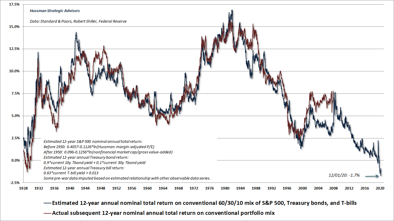
The charts below will help to convey the historic and breathtaking extremes that we presently observe in the financial markets. The first chart shows our estimate of prospective 12-year nominal total returns for a conventional portfolio mix invested 60% in the S&P 500 Index, 30% in Treasury bonds, and 10% in Treasury bills. This estimate is presently -1.7%, suggesting that investors are facing a very long trip to nowhere. The component with the poorest return estimate here is the S&P 500, at a projected -3.6% annual loss for the coming 12-year period, including dividends. The red line shows the actual subsequent 12-year return on this same portfolio mix, and of course ends 12 years ago since we don’t yet know the full-period returns for more recent points.

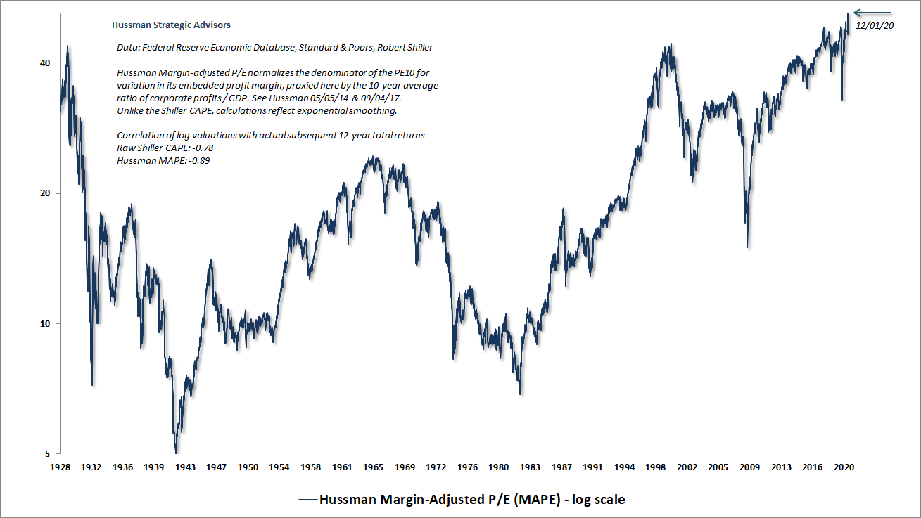
The chart below shows our Margin-Adjusted P/E (MAPE), which is better correlated with actual subsequent market returns than nearly every alternate measure we’ve tested or introduced. Currently, the MAPE stands at the most extreme level in U.S. history, eclipsing the extremes of 1929 and 2000.

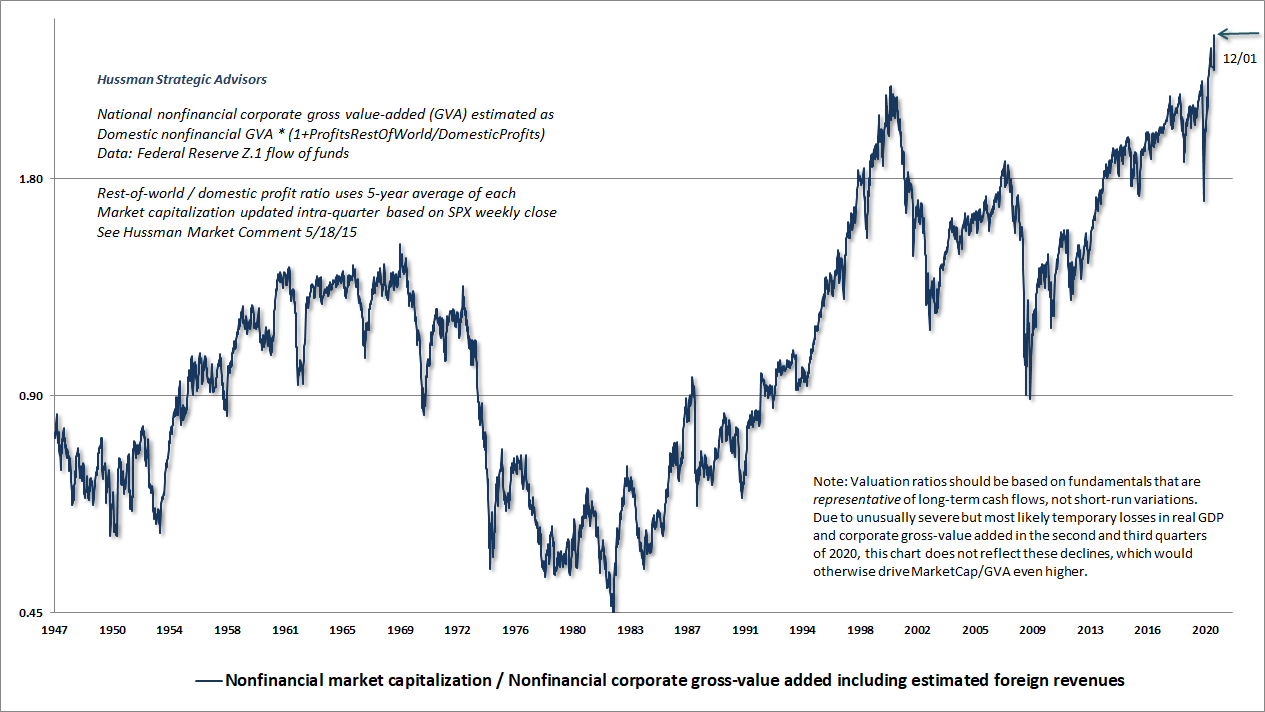
The chart below shows the ratio of MarketCap/GVA, which I introduced in 2015 and remains the valuation measure we find best-correlated with actual subsequent S&P 500 total returns across decades of complete market cycles. MarketCap/GVA measures nonfinancial market capitalization to corporate gross value-added, including our estimate of foreign revenues. Again, this measure stands at the most extreme level in U.S. history. It’s worth noting that because I believe that valuation measures should be based on fundamentals that are representative of very, very long-term future cash flows, neither the MAPE nor MarketCap/GVA reflect the downturn in economic activity during the second and third quarters of 2020, which would otherwise make both measures even more extreme.

Back in October 2002, as the economy was reeling from the collapse of the tech bubble, and the Fed was slashing interest rates toward the 1% level that would give rise to a housing bubble and a global financial crisis, Ben Bernanke gave a speech in which he tossed out this little chestnut: “First, the Fed cannot reliably identify bubbles in asset prices. Second, even if it could identify bubbles, monetary policy is far too blunt a tool for effective use against them.”

Look. When you eat, sleep, and dance on a zero-interest rate monetary accelerator for nearly a decade – perpetually encouraging yield-seeking speculation that drives reliable valuation measures to the most extreme levels in history – guess what? You’ve created a bubble. Perhaps the tools at the Fed are simply too blunt to recognize this.

Investors have become so intolerant of the frying pan of zero interest rates that they’re now only too willing to launch themselves into the fire. Speculation has now driven our estimate of prospective 12-year S&P 500 total returns to -3.6%.

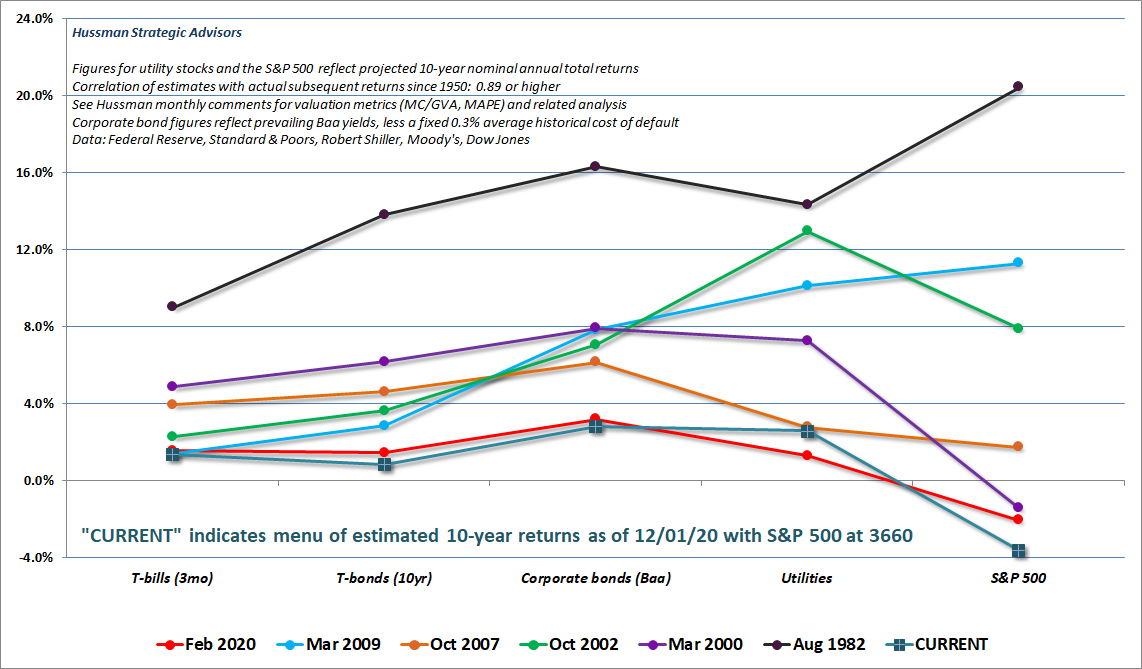
One way to see the “out of the frying pan and into the fire” behavior of investors here is to examine the profile of estimated investment returns across a broad range of investment assets, including T-bills, Treasury bonds, corporate bonds, utilities, and the S&P 500. Each line in the chart below shows our estimate of prospective returns on various asset classes at a particular point in time, where all of the underlying estimates have a correlation of 0.89 or higher with actual subsequent returns. The current profile is also the lowest.

If there’s one thing to notice about these profiles, it’s that they vary over time. The investment opportunity set is constantly changing. At present, investors have apparently decided that if they’re going to price bonds at levels that provide long-term returns of next-to-nothing, they might as well go ahead and price everything that way. When investors look back on this moment, I expect that they will remember this opportunity set as one of the worst of their lifetimes.

A very long, interesting trip to nowhere

Over the past 5 years, the revenues of S&P 500 technology companies have grown at a compound annual rate of 12%, while the corresponding stock prices have soared by 56% annually. Over time, price/revenue ratios come back in line. Currently, that would require an 83% plunge in tech stocks (recall the 1969-70 tech massacre). The plunge may be muted to about 65% given several years of revenue growth. If you understand values and market history, you know we’re not joking.”

– John P. Hussman, Ph.D., March 7, 2000

Presently, I expect that the completion of this market cycle is likely to involve a loss in the S&P 500 on the order of 65-70%. I realize, of course, that this sounds insane. The problem is that this projection is fully in line with a century of evidence, and is consistent with the extent of market losses that would be run-of-the-mill given present valuation extremes. Indeed, the only reason that the S&P 500 did not lose a similar amount during the 2000-2002 collapse (though the tech-heavy Nasdaq 100 lost a weirdly precise -83%) is that the market did not actually reach its valuation norms by the end of that cycle. Instead, the market went on to breach its 2002 bear market low during the 2007-2009 collapse. That’s when valuations finally moved to levels that I viewed as undervalued from the standpoint of historical norms (as I noted in late-October 2008).

The chart below provides some perspective about where the S&P 500 stands relative to its long-term valuation norms. Notice in particular that movements in the blue line (the S&P 500) well above the green valuation line tend to be transient, while market advances toward the green valuation line from below are typically not surrendered in later market cycles. It would take a roughly 67% market loss simply to reach that green line from here.

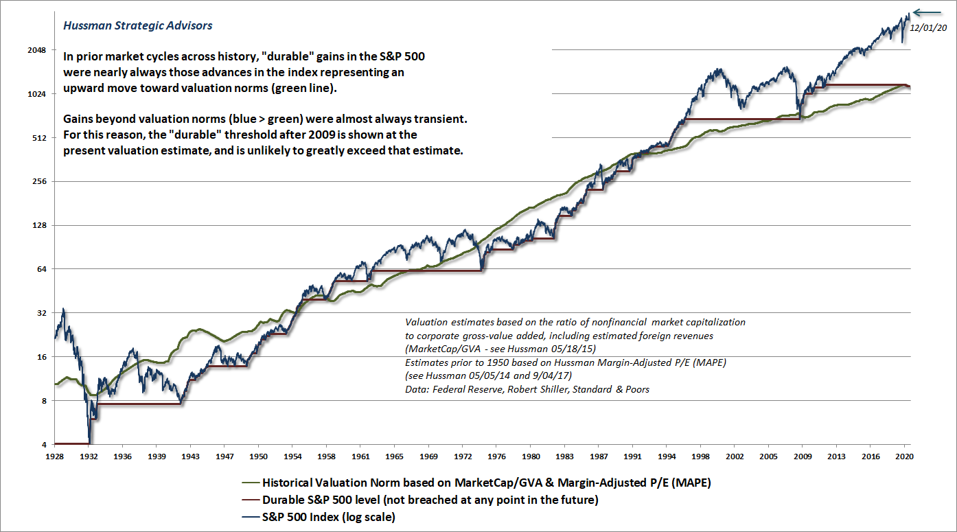
The chart above provides insight into why I view a very long trip to nowhere as likely in the years ahead. This analysis may also help to understand why the total return of the S&P 500 lagged Treasury bills for the entire period between May 1995 through March 2009, despite two intervening bubbles.

The stock market has experienced several long, interesting, but ultimately unprofitable trips to nowhere over the past century. These periods have either started at elevated valuations, ended at depressed valuations, or some combination of both. I have little doubt that measured from present valuation extremes, investors will look back at some future date, more than a decade from now, and find that they’ve lagged even the depressed yields available on Treasury bills.

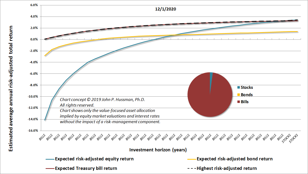
The chart below shows our “value-focused asset allocation” approach, which I described in a 2019 white paper. Note that this allocation does not reflect any modification based on the condition of market internals and other factors, but is instead driven purely by valuations. At present, the value-focused asset allocation assigns virtually nothing to the S&P 500 and nearly everything to Treasury bills. The last time the equity component was this low was during two weeks in the third quarter of 2007, as the market was peaking before the global financial crisis. The last time the Treasury bill component was this high was at the 1929 market peak, along with a 7-week period in March and April of 1930 as the market pushed to the recovery high that followed the 1929 crash, and preceded a further market loss of over 85%.

Safety nets and tail-risk hedges are essential

With regard to immediate, “local” market conditions, there’s no question that investors have had the speculative bit in their teeth in recent months. When investors are inclined to speculate, they tend to be indiscriminate about it, so we can gauge that psychological inclination based on the uniformity or divergence across thousands of individual stocks, sectors, industries, and security-types, including debt securities of varying creditworthiness.

Since our measures of market internals are consistent with speculative pressure, and because we abandoned, in late-2017, our belief that the recklessness of Wall Street has any natural limit, we have not fought the recent advance with an outright bearish stance. But conditions are certainly overextended and overbullish enough to encourage a neutral outlook rather than a constructive one, and I strongly believe that safety nets and tail-risk hedges are essential here.

It’s also worth noting that though unfavorable internals accompanied the February market peak, our measures of market internals can sometimes still be constructive at a market peak. That’s why extremely overvalued and overextended conditions can still encourage us to adopt a neutral outlook despite constructive internals. Present extremes don’t allow a positive market outlook here. But we are content to defer an outright bearish outlook until we observe some amount of deterioration and divergence.

Presently, we observe measures of overextension that have been rare outside of market peaks such as March 2000 and November 2007. To the extent that history is a guide, I expect that the initial loss from recent highs will be rather abrupt. As we saw even in late-2018 and early this year, first leg down tends to be steep and disorienting, and it becomes psychologically difficult to sell well below the highs. That’s what keeps many investors holding on as prices decline further. For our part, we’re content to maintain a “locally” neutral outlook, and to let our existing safety nets take care of larger downside risks more or less automatically.

The stock market has experienced several long, interesting, but ultimately unprofitable trips to nowhere over the past century. These periods have either started at elevated valuations, ended at depressed valuations, or some combination of both. I have little doubt that measured from present valuation extremes, investors will look back at some future date, more than decade from now, and find that they’ve lagged even the depressed yields available on Treasury bills – just as the total return of the S&P 500 lagged Treasury bills for the entire period between May 1995 through March 2009, despite two intervening bubbles.

George Soros used to get a back spasms just before the market suffered an abrupt break. My right leg starts unconsciously tapping like mad. I thought it might have been the pumpkin pie, but on further analysis, it’s because current market conditions are so familiar.

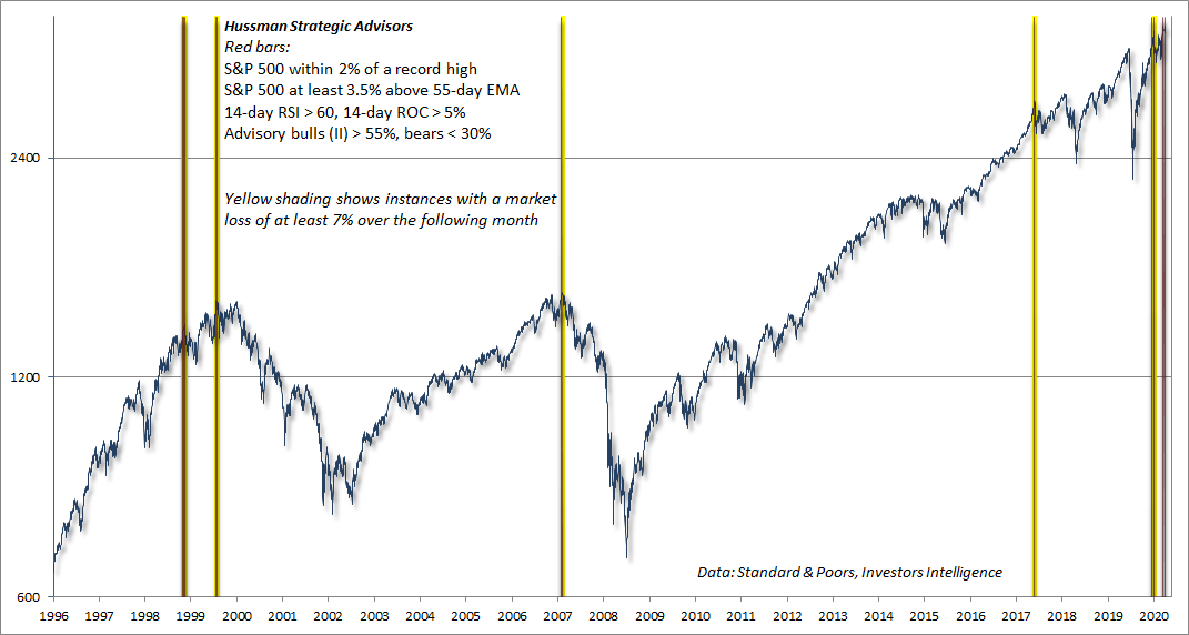
The red bars in the chart below show one of the more extreme syndromes of “overvalued, overbought, overbullish” conditions one can define. The specific conditions are shown in the chart text. The bars with yellow shading show instances where this syndrome has been in place, and the S&P 500 dropped at least 7% over the following month. All of these instances, prior to those of the past few days, are shaded yellow.

I should note that if one extends these criteria outside of the bubble period since the late-1990’s, one should include valuation criteria explicitly, along with some minimum advance from a 5-year low (most variants of “overvalued, overbought, overbullish” syndromes we track use 50-70% as a threshold). I prefer our MarketCap/GVA and MAPE as valuation measures, but even a Shiller P/E in excess of 18 (it’s currently near 34) will limit instances to periods that are actually overvalued.

The option value of cash

With our value-focused asset allocation encouraging the highest allocation to cash since 1929, aside from the peak of a post-crash correction in early-1930 that preceded the bulk of the 1929-1932 collapse, now seems to be an ideal time to explain why the interest rate on cash can be a poor measure of the value of cash (or hedged equity) as an investment alternative.

Let’s begin with two simple examples, and then we’ll formalize the idea.

The first case is extreme because it will provide some useful intuition. Suppose I offer you a security that will pay $100 two days from today. You can buy as much of it as you like today at $50, or you can wait until tomorrow. Tomorrow, I’ll flip a coin. If it’s heads, I’ll sell you the security at $99. If it’s tails, I’ll sell you the security at $25. What should you do?

Clearly, if you buy the security today, you’ll double your money two days from now. That’s a 100% expected return for each dollar you invest, over that 2-day period. If you wait, you’ll earn nothing on the first day, but you’ll then have two possibilities. If heads, you’ll get just 1% on your invested money. If tails, you’ll get a 300% return, quadrupling your money. With a 50/50 chance at each, your expected return for every dollar you invest is 0.5*1% + 0.5*300% = 150.5%. So waiting adds 50.5% to your expected return over that 2-day period. With an extreme example like this, risk aversion would undoubtedly be a consideration, but from an expected return perspective, and particularly if we repeat the game over and over, you’re clearly better off staying in cash on day one, despite the very high expected return from investing right away.

It’s tempting to say, “Now, hold on. The expected price tomorrow is 0.5*99 + 0.5*25 = $62, which is higher than $50, so I should obviously invest today.” But this argument overlooks that there are actually two distinct investment opportunities that you obtain by waiting. In one, you will quadruple the entire amount invested. In the other, you will gain just over 1% on the entire amount invested. Each of these has a probability of 50%. While the “expected” price in the second period is obviously $62, that price is emphatically not the actual opportunity you will face in the second period. Option value emerges because the act of waiting splits the second-period opportunity set in a valuable way. The potential benefit of obtaining a lower future price outweighs the potential cost of missing an immediate gain. In other words, waiting provides an option that would be lost by investing immediately, and that option has value.

Now let’s extend this to a less extreme example. Suppose that a security will deliver a single $100 payment a decade from today. Suppose the price of the security is $74.40. With that, you can quickly calculate that the 10-year expected return on the security is 3% annually. We’ll also assume that cash earns nothing.

Given these assumptions, it seems obvious that the security is a better investment than zero-interest cash. But hold on. Suppose that the security price is volatile enough that it might be 25% higher one year from now with a probability of 0.51, or 20% lower with a probability of 0.49. I’ve chosen those numbers so their expected value is still 3%. With that extra piece of information, it turns out that you’re actually better off holding cash and waiting to see what happens, even though cash provides a zero return.

Why is cash a more valuable option? Well, if you buy the security today, your cumulative return over the coming decade will be $100/$74.40 -1 = 34.41%, regardless of what happens next year.

But suppose you wait. The action of waiting gives you access to two possibilities. In the event of an upmove, which has a probability of 0.51, you’ll miss that gain, the new price will be $93.00 and your cumulative return at the end of the decade will be $100/93.00-1 = 7.53% if you invest at that point. But waiting also gives you the possibility of a 20% price decline, to $59.52, in which case your cumulative return at the end of the decade will be 68.01%. Weighting those two distinct outcomes by their probabilities, your expected cumulative return if you wait is 0.51*7.53% + 0.49*68.01% = 37.17%.

Given the low expected return on the passive investment, coupled with a reasonable level of volatility, it turns out that holding cash has an “option value.” You might miss out on the upmove, but you also gain the potential to invest at a lower price than is currently available. In this example, holding cash for a year, even at zero interest, actually raises your expected wealth at the end of the decade by 37.17% – 34.41% = 2.76% over a passive buy-and-hold approach.

By holding the security today, a passive investor can expect an average price next year of $76.59, a gain of 3% from the current price, and a level that would be expected to provide further gains averaging 3% annually over the following 9 years. But the passive investor loses the opportunity to take advantage of potentially better returns that a decline might produce. The risk is missing out on a potential gain. That risk is highest when the security is reasonably valued and likely to produce acceptable returns, and lowest when the security is richly valued already and has a small expected return. So the option value of cash is highest when the investment security is at high valuations that imply relatively small returns, and when the security is also subject to volatility.

It’s worth noting that sufficiently high volatility can increase the option value of cash, even if a security is undervalued. However, cash stops having compelling option value when the expected return on the security is high, and volatility and risk-aversion begin to recede. That’s as good an explanation as any for why the strongest market return/risk profiles we identify are associated with a significant retreat in valuations that is then joined by an improvement in our measures of market internals.

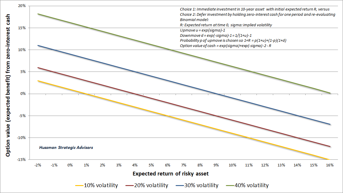
We can formalize our intuition about the option value of cash in a precise way. I’ve spared you the arithmetic, but the details are embedded in the chart text below. I’ve framed the expected value of holding cash within a simple binomial pricing model, though it differs from certain other formulations by recognizing that every security is a claim to a discounted stream of future cash flows, and not just some untethered lottery ticket fluctuating under Brownian motion.

The basic idea is this: when the expected return of a given security is low, zero interest cash can dominate a passive investment decision, even if volatility is fairly low as well. As the expected return of the security rises, higher levels of volatility are required in order to justify holding zero-interest cash instead of the asset.

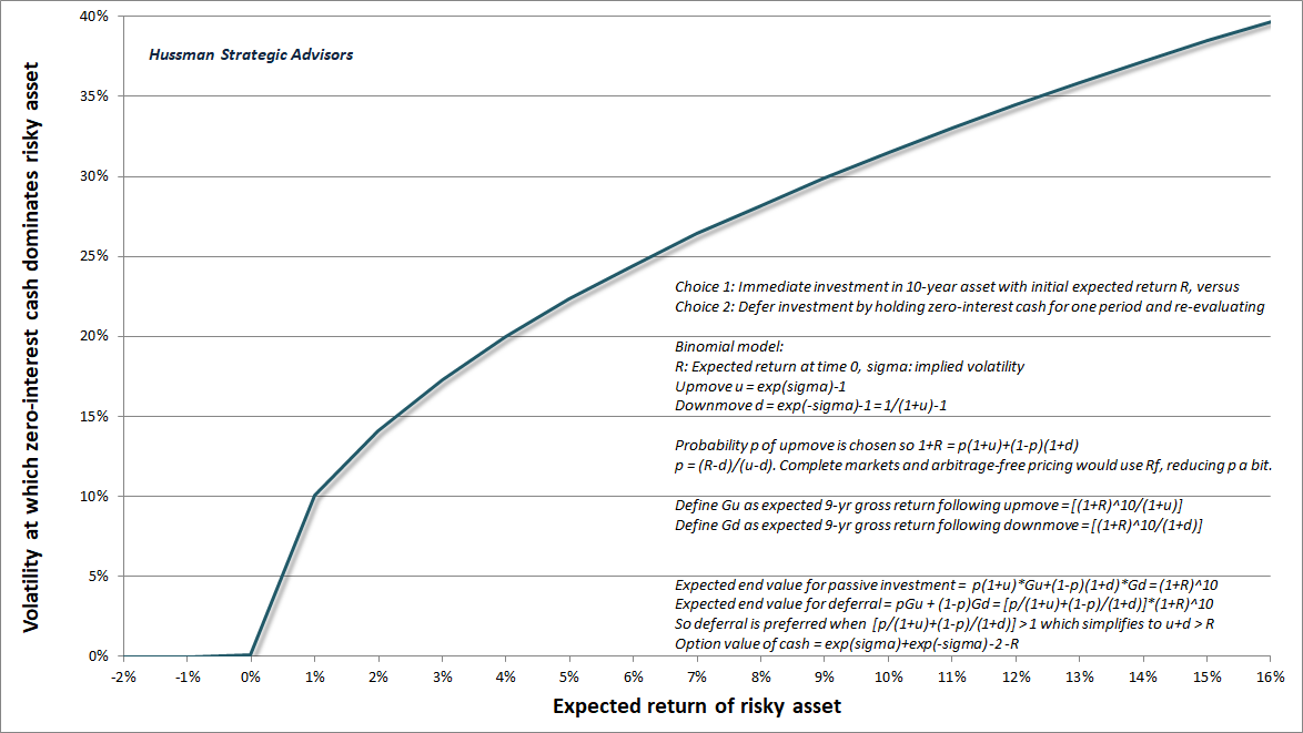
Stated another way, given the choice of investing in a risky security, or holding cash in the hope of better opportunities, the “option value of cash” is greatest when a) the expected return of the security is low, and b) the potential volatility of the security is high.

All of this has enormous relevance for the current stock market. By our estimates, the likely return of the S&P 500 over the coming 12-year period is actually a loss of -3.5% annually. That alone actually makes zero-interest cash a competitive alternative, in my view. But the case for cash (or our preference, hedged equity) is far more compelling, because the lowest prospective S&P 500 expected returns in history are also coupled with the potential for one of the deepest market losses on record over the completion of this cycle.

The chart below illustrates the relationship between valuations and subsequent market drawdowns. The blue line shows S&P 500 valuations, as measured by MarketCap/GVA, where valuations are inverted and truncated at their historical norm. So the lower that blue line is, the more extreme valuations have become. The red shaded area shows the largest S&P 500 drawdown over the following 3-year period (right scale). You’ll notice that extreme valuations aren’t always immediately associated with drawdowns. That’s why you see those white spaces between the blue valuation lines and the red drawdown areas, which occur during periods when a bubble is expanding. Unfortunately, the drawdowns generally arrive with a vengeance. At present, we expect the current cycle to be completed by a market loss on the order of 65-70%.

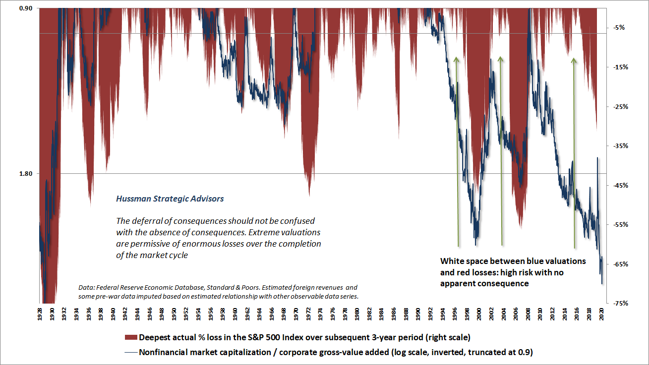
Yes, I know. A drawdown of 65-70% sounds insane and utterly preposterous, but the revulsion to that idea is largely due to pervasive speculative psychology, not historical evidence, cash flows, or fundamentals. From the standpoint of fundamentals, the most reliable set of valuation measures we’ve tested across a century of market cycles place current valuations at roughly 3.3 times the run-of-the-mill norms from which historically normal market returns have actually emerged.

Given the choice of investing in a risky security, or holding cash in the hope of better opportunities, the ‘option value of cash’ is greatest when a) the expected return of the security is low, and b) the potential volatility of the security is high.

Having abandoned the idea that speculative recklessness has a limit, we cannot, and need not, rule out a “permanently high plateau” in valuations. But one should recognize that such a plateau would still likely be associated with long-term market returns in the low single digits, coupled with above-average volatility. That’s because when valuations are elevated, even very small changes in expected returns correspond to rather large price fluctuations. After all, how do you raise an S&P 500 dividend yield of just 1.6% to a dividend yield of just 2%? You cut prices by 20%. How do you move from the single highest MAPE and MarketCap/GVA in history to the highest 4% in history? You cut prices by 20%.

All of that takes us back to a situation where cash has option value. But it’s also a situation where it will remain useful to regularly monitor the condition of market internals. In particular, I expect the strongest investment opportunities to emerge in periods where a material retreat in valuations is joined by favorable uniformity in market internals, while the most hostile investment environments will likely be those where extreme valuations are coupled with overextended conditions and emerging deterioration in our measures of internals. As usual, we’ll respond to that evidence as it emerges.

Inflation will not bail out a hypervalued market

While I expect that our attention to valuations, market internals, overextended conditions and the like will help us to navigate the coming market cycles regardless of how the course of inflation unfolds, it’s at least worth mentioning that inflation is not likely to benefit stocks at these valuations, or provide a meaningful offset to the downside risk we expect over the completion of the market cycle.

Across a century of U.S. data, the total return of the S&P 500 has significantly lagged Treasury bills during periods when inflation has been anywhere above about 2% and rising. The comparison has been particularly hostile to the S&P 500 when the year-over-year CPI inflation rate has been anywhere above about 3.2%, and higher than its level of 6 months earlier.

The first casualty of rising inflation is market valuations. It’s only after valuations have been driven to historically normal or below-average levels that the positive effect of inflation on nominal cash flows dominates the negative impact on valuations. So yes, if inflation is rapid enough, the effect on nominal values can eventually dominate. But given present valuation extremes, that outcome would currently require the consumer price index to more than triple first.

The effect of inflation in boosting nominal stock market returns is more immediate if valuations begin at depressed levels, as they did in the early 1940’s. In contrast, the economy can sustain quite a bit of inflation without benefit to stocks if valuations begin at elevated levels, as they did in the early 1970’s. Regardless, when we examine the two 10-year periods having the highest trailing CPI inflation rates (the decades ending in March 1951 and September 1981), we find that the 10-year total return of the S&P 500 during those periods fell short of could have been projected simply based on prevailing valuations at the beginning of those periods.

Put simply, U.S. stocks have actually earned their reputation as “inflation hedges” in periods when inflation is falling, starting valuations are depressed, or both. Once valuations have been crushed, stocks recover lost ground – particularly once the rate of inflation has peaked and begins to normalize. The combination of depressed starting valuations and falling inflation is exactly what contributed to the enormous stock market returns during the disinflationary period between the early 1980’s and the 2000 bubble peak.

The current environment could not be further from that set of conditions.

The Fed, the Treasury, and future policy directions

Overall, I’m encouraged by the economic team announced by the incoming Biden-Harris Administration, which seems inclined toward economic supports that can directly benefit ordinary families and targeted investment, instead of relying on trickle-down fiscal policies and distortive monetary policies. I expect a greater focus on infrastructure, alternative energy, equitable growth, and initiatives likely to benefit the average American. From my perspective, that will be a welcome reversal from years of treating overvalued financial markets as sacrosanct objects of policy, and initiatives that have been far more concerned with financial “capital” (i.e. profits and securities) than with productive capital (i.e. tangible investment).

Given the extent to which Janet Yellen dismissed the idea of the Fed altering its policy course in response to the escalating housing bubble in late-2005 (“My answers to these questions in the shortest possible form are ‘no,’ ‘no,’ and ‘no.’”), and given the extent to which the Yellen Fed amplified yield-seeking speculation in the recent bubble, restricting attention only to the objects of Phillips Curve dogma despite growing financial distortions, it will be no surprise that I was disappointed by the choice of Janet Yellen at Treasury. It’s impossible to identify a meaningful effect of activist monetary policies on employment gains, beyond the run-of-the-mill mean-reversion that has always followed recession lows regardless of the Fed’s policy stance. Activist monetary policy is certainly not worth the speculative distortions, malinvested savings, financial crises, and employment losses that inevitably follow.

I expect that in the next few years, Janet Yellen will likely find herself in the rather uncomfortable position of having to eat her own cooking. I will certainly wish her the best, but I’ll also speak as loudly as possible against policy responses that would use public funds to bail out private investment losses. With valuations at over three times their historical norms, it will be a long way down before bailout funds used in that fashion would represent useful “investments” on behalf of the American public, whether administered by the Fed or by the Treasury.

As for the decision of the current Treasury to withhold remaining CARES funds that were allocated to the Fed for the purpose of emergency loans, I actually welcome that decision. The Fed was always poorly-equipped to implement these efforts. My preference had been for a far different structure, comprising mainly emergency funding directed to the entry point of the circular flow. So in addition to direct support for households, support for businesses would better have taken the form of both PPP loans and refundable tax credits, but with a much different structure than in CARES.

Specifically, public support and loan forgiveness should have been contingent on actual economic damage. If you weren’t damaged, you shouldn’t be receiving public money. Here’s the basic structure that I proposed when CARES legislation was being constructed. It turned out that even getting simple Congressional oversight of how the funds would be used was nearly impossible. Still, I think the considerations I detailed earlier this year remain important for the next round:

Set a “basic income” threshold that creates a uniform playing field, regardless of whether an assistance program involves unemployment compensation, payroll protection program (PPP) loans, or even loans to large corporations. A reasonable model might be some minimum income level, plus some percentage of an individual’s median payroll income over the past 3 years, with the basic income capped at, say, one or two times U.S. median personal income, above which public funds would not subsidize.

Then, for any company receiving public support, loans would be forgiven only to the extent that the company shows an “adjusted loss.” Adjusted loss meaning that one would examine the company’s net income or loss for 2020, and then disallow from expenses any excess compensation paid to management or employees above their “basic income” amount, as well as any expenses incurred for unused inventory, prepayments, items that don’t represent 2020 operating costs, or expenses in excess of say, the prior 3-year high. If the company still has a loss after those adjustments, then fine, a portion or the entirety of the loan could be forgiven. Instead of the Fed, The IRS could administer support through existing SSN (individuals) and EIN (businesses) registrations, and would be most capable of applying criteria related to loan forgiveness or recovery.

Finally, remember that the moment the government runs a “deficit,” there is absolute certainty that at least one other sector – households, corporations, or foreign countries – will run a “surplus,” in which the income of that sector will exceed its consumption of U.S. goods and services and net real investment (e.g. homes, buildings, capital equipment). The structure of an economic package affects which sector accrues the private ‘surplus’ associated with government deficits.

Here’s some arithmetic that may help to conceptualize how the deficit of one sector emerges as the surplus of another. It’s actually an accounting identity:

Government consumption expenditures, net investment, and transfer payments – Government tax revenue = Household after-tax income not spent on consumption or real net household investment + Undistributed after-tax corporate profits not used for real net corporate investment + Foreign income due to the U.S. trade deficit (i.e. imports – exports)

If we want deficits to benefit families, and to encourage productive private and public sector investment, that’s where we should target our policies. It’s madness to use public funds to subsidize the private losses of speculators. It’s madness to bail out bondholders instead of facilitating packaged restructurings that preserve ongoing employment and activity by haircutting the bad debt. It’s madness to provide private and corporate tax benefits and subsidies in hope that they will trickle down to the masses, with zero accountability for actually doing so.

As it happened, the various programs overseen by the Fed ultimately allocated only about $88 billion of CARES funding. About $58.6 billion of that was allocated to the Paycheck Protection Program Liquidity Facility, which provides liquidity to banks, using their PPP loans (which are administered by the Small Business Administration) as collateral. Note that this is a bank liquidity program. It doesn’t finance the actual PPP loans, which exceeded $500 billion using CARES funds provided through the SBA.

Among other Fed programs, the total allocated by the Fed to the Main Street and Municipal lending programs amounted to just $6.7 billion. That’s just half of the $13.5 billion that the Fed allocated to secondary market purchases of unbacked corporate debt. Even those bond purchases were a drop in the bucket in an economy where nonfinancial corporate debt alone amounts to $7.1 trillion. The Fed did also make $3.7 billion in loans through its Term Asset-Backed Loan Facility (TALF), which were more appropriately collateralized by AAA asset-backed securities.

Every dollar created by the Fed must be backed by government securities or by collateral “sufficient to protect taxpayers from losses”. Even the notion of the Fed using public funds to buy unbacked corporate securities from investors is quite dangerous, so let’s be clear that the outright purchase of outstanding, unsecured corporate debt from investors, no strings attached, violated the intent of CARES 4003(c)(3)(B) and Federal Reserve Act 13(3). When the legislative wording literally includes the phrase “for the avoidance of doubt,” one can be reasonably sure that one is reading the intent of the law. Unfortunately, this needs to be spelled out like a children’s book. Congress should be careful to prohibit the Fed from “lending” to “special purpose vehicles” that use public funds to buy unbacked corporate securities, and to then treat the unbacked securities held by the SPV as if they are actually “collateral” in any meaningful sense of the word.

As a practical matter, it’s possible to scrape enough grey areas out of the legislative wording of the CARES Act to argue that the Fed’s purchases of corporate bonds were allowed by 4003(b)(4)(B), but even that strained argument holds only for purchases financed directly by funds provided by the Treasury, and where those Treasury funds themselves could be interpreted as the 13(3) “collateral.” It’s a major red flag that the Fed counted the unsecured bonds as collateral as well, and that it booked them at cost rather than market value, because that’s like claiming that any unbacked IOU scribbled on a napkin can be treated as its own collateral.

In any case, the use of additional Fed “leverage” would have been patently illegal, and it seems that the Fed understood this because leverage (i.e. creating base money to buy unbacked corporate bonds beyond the amount of funding approved and provided by Congress) was never used, as far as I can tell. In addition to $8.5 billion in corporate bond ETFs, the Fed’s “secondary market corporate credit facility” holds about $5 billion in individual bonds. As of 11/24/20, the largest holdings were, in order: AT&T, Volkswagen Group of America Finance, Toyota Motor Credit, Daimler Finance North America, Verizon, Apple, Comcast, and BMW US Capital. Over 74% of the dollar value in the top 4 holdings represented bonds issued by wholly-owned subsidiaries of foreign companies. This is what one gets when one places the Federal Reserve in charge of allocating funds on behalf of the American public. We can do better.

---

---

The foregoing comments represent the general investment analysis and economic views of the Advisor, and are provided solely for the purpose of information, instruction and discourse.

Prospectuses for the Hussman Strategic Growth Fund, the Hussman Strategic Total Return Fund, the Hussman Strategic International Fund, and the Hussman Strategic Allocation Fund, as well as Fund reports and other information, are available by clicking “The Funds” menu button from any page of this website.

Estimates of prospective return and risk for equities, bonds, and other financial markets are forward-looking statements based the analysis and reasonable beliefs of Hussman Strategic Advisors. They are not a guarantee of future performance, and are not indicative of the prospective returns of any of the Hussman Funds. Actual returns may differ substantially from the estimates provided. Estimates of prospective long-term returns for the S&P 500 reflect our standard valuation methodology, focusing on the relationship between current market prices and earnings, dividends and other fundamentals, adjusted for variability over the economic cycle.