

Always a Reckoning


John P. Hussman, Ph.D.
President, Hussman Investment Trust
April 2021
In 1965, arithmetic indicated expectation of a much lower rate of advance in the stock market than had been realized between 1949 and 1964. That rate had averaged a good deal better than 10% for listed stocks as a whole, and it was quite generally regarded as a sort of guarantee that similarly satisfactory results could be counted on in the future. Few people were willing to consider seriously the possibility that the high rate of advance in the past means that stock prices are ‘now too high,’ and hence that ‘the wonderful results since 1949 would imply not very good but bad results for the future.’
– Benjamin Graham, The Intelligent Investor, Fourth Revised Edition, 1973
From 1949 through 1964, the S&P 500 enjoyed an average annual total return of 16.4%. In the 8 years that followed, through 1972, the total return of the index averaged a substantially lower 7.6% annually; strikingly close to the 7.5% projection that Graham had suggested based on prevailing valuations, yet still providing what Graham had suggested would likely “carry a fair degree of protection” against inflation, which averaged 3.9% over that period.
Graham was much less favorably inclined toward stocks by 1972, suggesting that “bond investment appears clearly preferable to stock investment.” During the full period from the 1972 market high to the 1982 market low, the S&P 500 actually declined in price, but enjoyed a 4.1% annual total return, entirely from dividend income. By comparison, both Treasury bill returns and U.S. CPI inflation averaged 9.0% annually. Meanwhile, Treasury bonds enjoyed a total return of 6.5% annually, which could of course be read directly from their yield-to-maturity at the beginning of the period.
The arithmetic of total returns
Value investing is at its core the marriage of a contrarian streak and a calculator.
– Seth Klarman
I’ve regularly noted that a good valuation measure is nothing but shorthand for a proper discounted cash flow analysis. In general, the denominator of a useful valuation measure should act as a “sufficient statistic” for decades and decades of future cash flows – that’s one of the reasons that earnings-based measures tend to be less reliable, while the valuation measures having the strongest correlation with actual subsequent market returns across history are those that have fairly smooth denominators that closely track corporate revenues.
The only way to hold a valuation ratio constant is for the numerator and the denominator to grow (or shrink) at the same rate. This is a useful fact for investors, because it allows us to break investment returns into underlying components that drive returns. This is the “arithmetic” that Graham describes in the opening quote above.
An example will make this arithmetic clear. During the 21 years since the bubble peak in 2000, S&P 500 revenues have grown at an average annual rate of about 3.5% annually. If the price/revenue ratio of the S&P 500 had remained fixed at its 2000 high of 2.36, that’s also the rate at which the S&P 500 Index would have gained. Instead, the price/revenue ratio closed last week at 3.09, the highest level in history. That change in valuations was worth another (3.09/2.36)^(1/21)-1 = 1.3% in annual return. Add an average dividend yield of about 2% during this period, and one would estimate that the total return of the S&P 500 should have averaged about (1.035)*(1.013)-1 + .02 = 6.8% annually. That estimate matches the actual return of the S&P 500.
The chart below shows the price/revenue ratio of the S&P 500 (log scale)
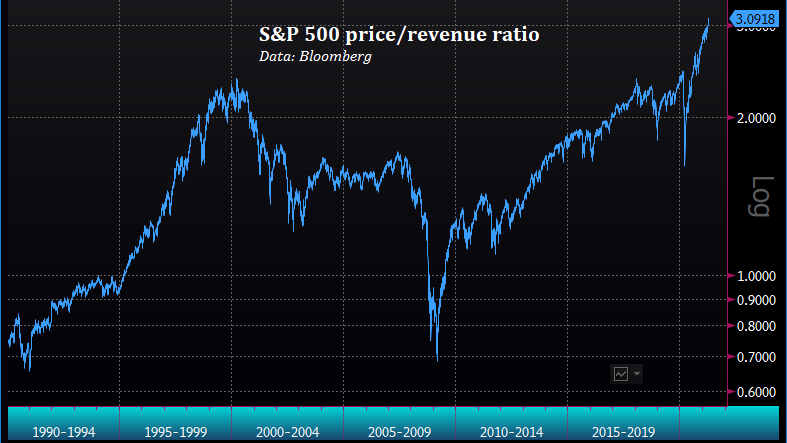
The problem is that the arithmetic of total returns can also swing wildly into reverse.
For example, in the 9 years from the bubble peak in 2000 to the market trough in 2009, S&P 500 revenues grew at an annual rate of 4.8% annually. Meanwhile, however, the price/revenue ratio of the index collapsed from 2.36 to just 0.68. That change in valuations created a drag of about (0.68/2.36)^(1/9)-1 = -12.9% annually on total returns. Add an average dividend yield of about 1.7% during that period, and one would estimate that the total return of the S&P 500 should have averaged about (1.048)(0.871)-1+.017 = -7.0% annually. Again, that estimate matches the actual return of the S&P 500.
Put simply, the total return that investors can expect breaks into exactly three components: the growth rate of fundamentals (where a smooth and fairly predictable fundamental is preferable), the annualized change in the valuation multiple (where a historically reliable measure is preferable), and the average dividend yield over the holding period.
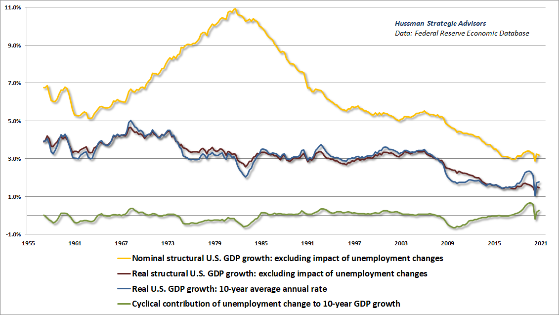
What does this arithmetic look like today? Consider first that both S&P 500 revenues and nominal GDP have grown at less than 4% annually over the past 10 and 20 years, and that the “structural” growth rate of real GDP – the growth of the economy excluding the effect of changes in the unemployment rate – has gradually slowed in recent decades to just 1.6% annually. Given that real structural growth isn’t highly variable, even 2% inflation would likely keep nominal growth around 4% annually. Moreover, valuations are typically the first casualty of inflation. As we observed in the 1970’s – stocks have been useful hedges against inflation only after valuations have first been crushed, and typically only when the rate of inflation is declining. So while faster inflation might boost nominal growth, it would also be expected to decimate valuations.
The chart below shows how U.S. real and nominal GDP growth rates have slowed over time, and the underlying contribution of structural and cyclical components.
If we assume that the current S&P 500 price/revenue ratio of 3.09 will remain at the current record level permanently, then 4% revenue growth would also translate into 4% price growth. Add the 1.4% dividend yield of the S&P 500, and a “permanently high plateau” in market valuations could reasonably be expected to result in average annual total returns of 5.4%.
The next question is how sensitive those returns would be to any failure of valuations to maintain a permanently high plateau. Well, let’s do the math.
Suppose that, despite trading below the 2000 price/revenue multiple of 2.36 as recently as last July, the S&P 500 never breaks below that 2000 peak valuation again. Instead, let’s even assume that it takes a decade simply for the current 3.09 multiple to retreat to 2.36. In that case, with 4% nominal growth and a 1.4% yield, one can estimate that the average S&P 500 nominal total return over the coming decade would be:
(1.04)*(2.36/3.09)^(1/10)-1 +0.014 = 2.6% annually.
Allow the S&P 500 price/revenue multiple to retreat, but never again lower than the 1.71 multiple observed at the October 2007 market peak, just before the global financial crisis, and the 10-year S&P 500 nominal total return could be expected to average:
(1.04)*(1.71/3.09)^(1/10)-1 + 0.014 = -0.6% annually.
Put simply, the total return that investors can expect breaks into exactly three components: the growth rate of fundamentals (where a smooth and fairly predictable fundamental is preferable), the annualized change in the valuation multiple (where a historically reliable measure is preferable), and the average dividend yield over the holding period.
All of this is a problem given that the historical norm for the S&P 500 price/revenue ratio is actually less than 1.0. Extreme starting valuations tend to be associated with very long periods in which the stock market goes “nowhere in an interesting way.” For example, allow valuations simply to touch their run-of-the-mill historical norm, even 20 years from today, without ever breaking below that norm (as it did in 2009). Add a 1.4% dividend yield, and the 20-year S&P 500 nominal total return could be expected to average:
(1.04)*(1.0/3.09)^(1/20)-1 + .014 = -0.3% annually.
Of course, we can form the similar estimates with numerous other measures. The key requirement is that the valuation measure should actually be highly correlated with actual subsequent market returns in decades of market cycles across history.
Across all of the valuation measures we’ve tested or introduced over time, the chart below shows where the most reliable among them stand at present. Each line is shown relative to its own history, so 1.0 represents the historical norm for each.
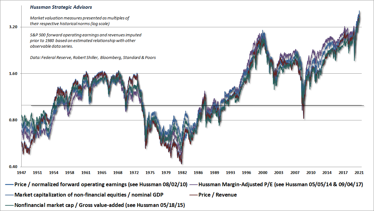
I heard a recent data-free suggestion that valuations might have been several times higher in the early 1900’s than at present. Given that the most reliable valuation measures tend to move roughly in tandem, the extended history in the chart below should be sufficient to disabuse such misconceptions.
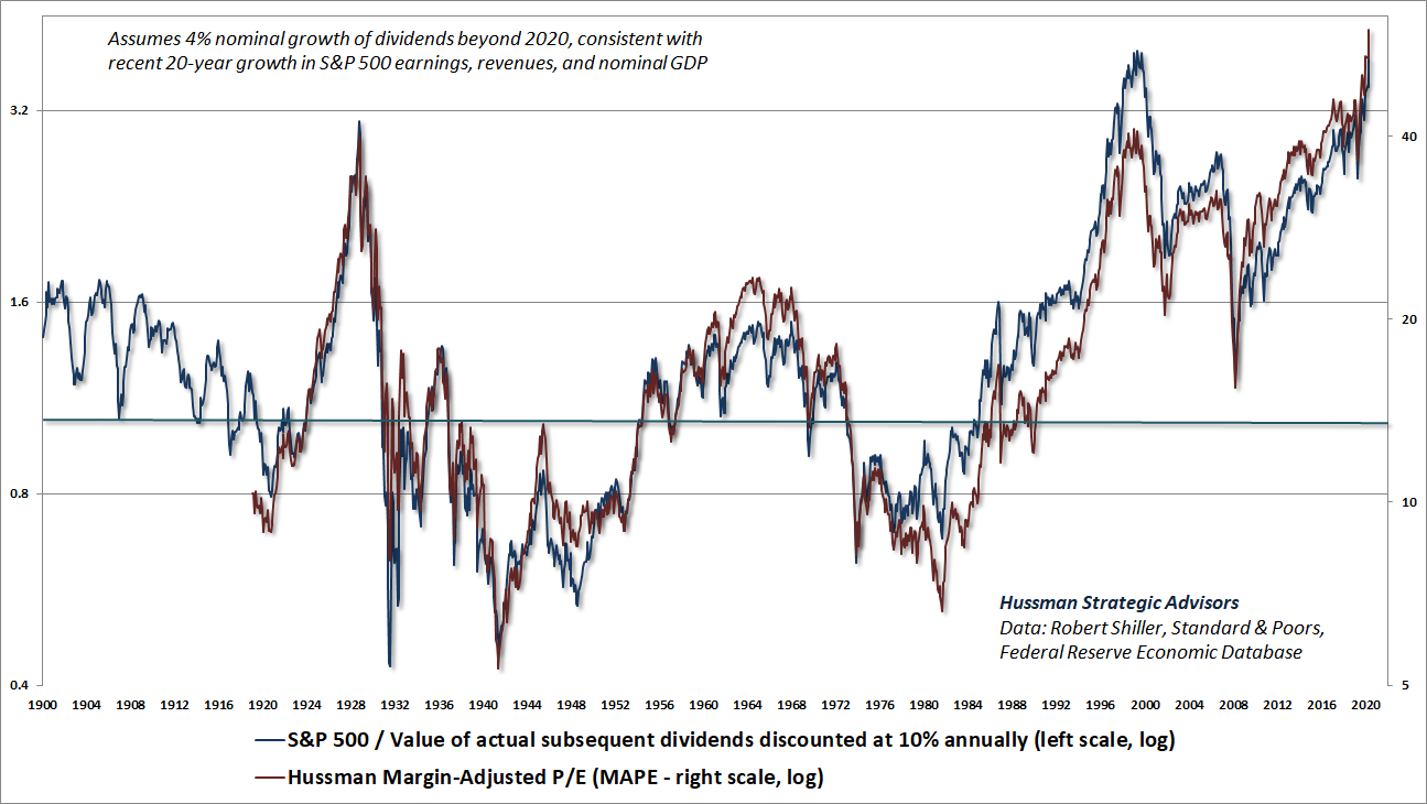
The red line shows our Margin-Adjusted P/E (MAPE), which is among the handful of measures we find best correlated with actual subsequent market returns across history. The chart also illustrates the fact that a good valuation measure is nothing but shorthand for a proper discounted cash flow analysis. The blue line shows what I’ll call our “Price/DDV” ratio for the S&P 500. The discounted dividend value (DDV) at each point in time is computed by discounting the stream of actual subsequent per-share S&P 500 dividends (which include the impact of stock buybacks) at a fixed 10% rate of return. One can use other rates of return, but 10% probably the most commonly assumed figure for “historically normal” returns.
What matters here to use a fixed rate, because then, a Price/DDV ratio of 1.0 implies that the S&P 500 is priced at a level that is consistent with long-term expected returns of 10%, while any deviation of Price/DDV from 1.0 means that the S&P 500 is priced for long-term expected returns different than 10%. As I’ve noted above, an expected growth rate of 4% is consistent with structural GDP growth as well as growth in S&P 500 revenues over the past two decades. One could choose a growth rate ignores this evidence, but even if growth was restored to the post-war average, the current multiple would count among the highest 4% of historical valuations, and it’s rather doubtful that interest rates would remain near zero.
A good valuation measure is nothing but shorthand for a proper discounted cash flow analysis
Meanwhile, it’s useful to understand how interest rates, growth rates, and valuations are related. Specifically:
- If the growth rate of fundamentals is held constant, saying that low interest rates “justify” high valuations is identical to saying that low expected returns on bonds “justify” low expected returns on stocks. Elevated valuations still imply depressed returns on stocks – investors just agree that those depressed returns are okay (or simply ignore that reality altogether).
- If interest rates are low because growth is also low (the two often go hand-in-hand), no valuation premium is justified at all. Future stock returns will be low anyway because of the depressed growth rate (e.g. consider P = D/k-g).
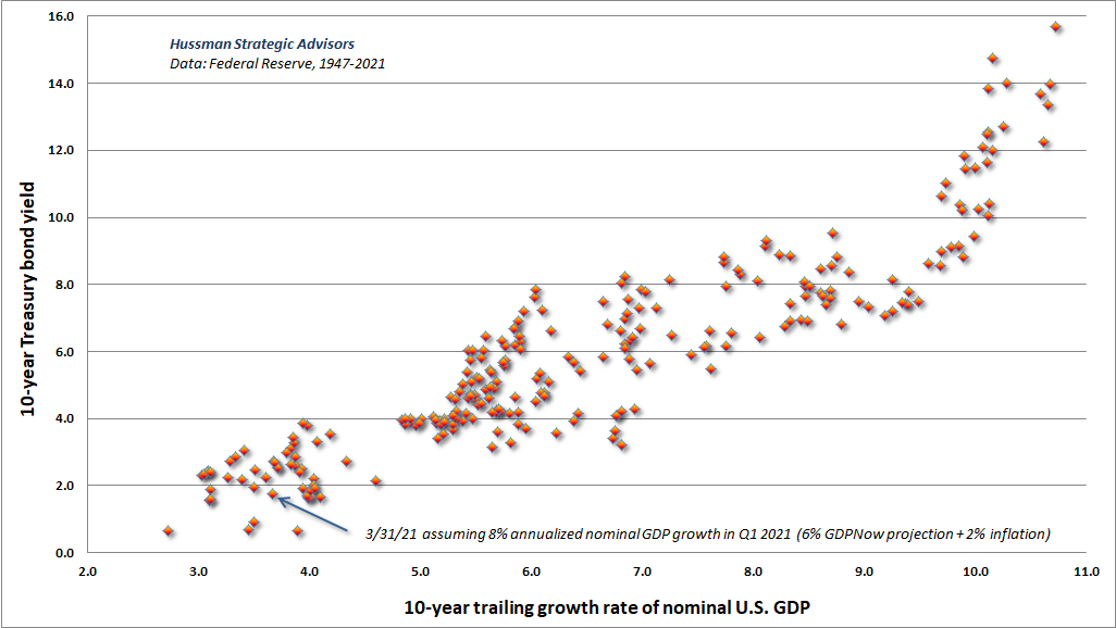
The chart below provides an overview of how GDP growth and interest rates have been related across history. In my view, the current depressed level of growth and the current depressed level of interest rates go hand in hand. The result is that no valuation premium is actually required in order to reduce the expected return of stocks to a level that is “justified” by low interest rates. The low rate of growth does that all by itself. To price stocks at record valuations here just adds insult to injury.
Divergent market internals and other high-risk conditions
There’s no question that speculative psychology can support valuations over extended segments of the market cycle. In our own discipline, we gauge that psychology based on the uniformity or divergence of market internals across thousands of stocks, industries, sectors, and security-types, including debt securities of varying creditworthiness. Those measures deteriorated in late-January. The bond market components deteriorated first, but we’re also monitoring early deterioration in leadership, breadth, participation, and price-volume behavior across a wide range of stocks. Meanwhile, we’ve been careful not to “fight” the residual speculative psychology too strongly.
My impression is that the next material market decline may take the form of a 25-35% air-pocket, driven by nothing more than the sudden concerted effort of overextended investors to sell, and the need for a large price adjustment in order to induce scarce buyers to take the other side. Such a decline would not require a recession. My current concerns are driven far less by economic factors than by the combination of valuations, leverage, and the potential for imbalanced order pressure. With regard to the economy, I do expect some “reopening” strength, but I also believe that this prospect has been extensively priced into valuations.
My friend Albert Edwards across the pond correctly notes that the ISM gauges are diffusion indices calculated by the percentage of respondents expecting the future to improve minus the percentage expecting the future to worsen. “These blockbuster ISMs should be treated with some caution – because if after an economy has been shut down every respondent thought things would be getting even a little better, then the ISMs would register the 100% maximum.”
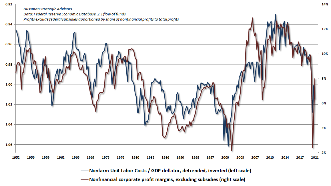
It’s also not at all clear that investors appreciate how much of the stability of corporate profits over the past year has been the direct result of government subsidies. If they did, they would also recognize that rising unit labor costs continue to place more pressure on corporate profit margins than the raw profit figures indicate. The chart below is one that I’ve presented before, showing the inverse relationship between U.S. nonfinancial profit margins and real unit labor costs. The only change below is that the impact of federal subsidies has been excluded.
Even if one wishes to take corporate profits at face value, it’s notable that the S&P 500 price/record earnings ratio currently stands at 29.4, easily above the 1929 peak of 22.8, and above every prior extreme in history except 1999-2000 (when profit margins were substantially below average). I introduced this measure 1998, in order to avoid uninformative spikes in the P/E due to weak earnings during periods of economic weakness. The ratio compares the S&P 500 with the highest level of earnings reported to date. It’s not our favorite valuation measure, but it’s clear that even an immediate return to record S&P 500 earnings would not support a positive view of market valuations. By the way, the same extremes are evident if one uses estimated “forward operating earnings,” though some imputation is required for historical data since Wall Street only created this concept in the 1980’s.
As usual, no forecasts are necessary, and we’ll defer our bearish outlook if we observe improvement in our measures of market internals. It’s enough to align our stance with the evidence as it arrives.
Always a reckoning
There always seemed to be a need
for reckoning in early days.
What came in equaled what went out
like oscillating ocean waves.
– Jimmy Carter, Always a Reckoning (excerpt)
From 1949 through 1964, U.S. nonfinancial corporate revenues grew at an average annual rate of 6.3% annually, and the dividend yield of the S&P 500 averaged 4.5%. Had market valuations remained constant, the total return of the S&P 500 would have averaged about 10.8% annually. Yet the actual total return was 16.4% annually, reflecting the benefit market valuations that more than doubled during that period (primarily during the 12-year span beginning in 1949, which will be important below).
As Benjamin Graham noted about stock market returns during that period, “That rate had averaged a good deal better than 10% for listed stocks as a whole, and it was quite generally regarded as a sort of guarantee that similarly satisfactory results could be counted on in the future. Few people were willing to consider seriously the possibility that the high rate of advance in the past means that stock prices are ‘now too high,’ and hence that ‘the wonderful results since 1949 would imply not very good but bad results for the future.”
As it happened, the total return of the S&P 500 would lag Treasury bills for a 20-year period from 1965 to 1985.
Graham’s point was essentially that, if past returns are substantially higher than one would have expected (based on valuations at the beginning of the period), it doesn’t mean that valuations are somehow broken or have “stopped working.” Rather, it’s an indication – even a confirmation – that current valuations may be extreme, and that future returns are likely to be disappointing. There’s always a reckoning.
The chart below shows the ratio of nonfinancial market capitalization to nominal GDP. While some of our other measures are more reliable, this measure certainly doesn’t deserve the dismissive attitude that many people on Wall Street have adopted toward it. The main issue is that there is a large “error” between the projection that one would have made in 2009 and the actual subsequent total returns of the S&P 500 over the following 12-year period. There are a few other “errors” like this as well. Investors would do well to understand them.
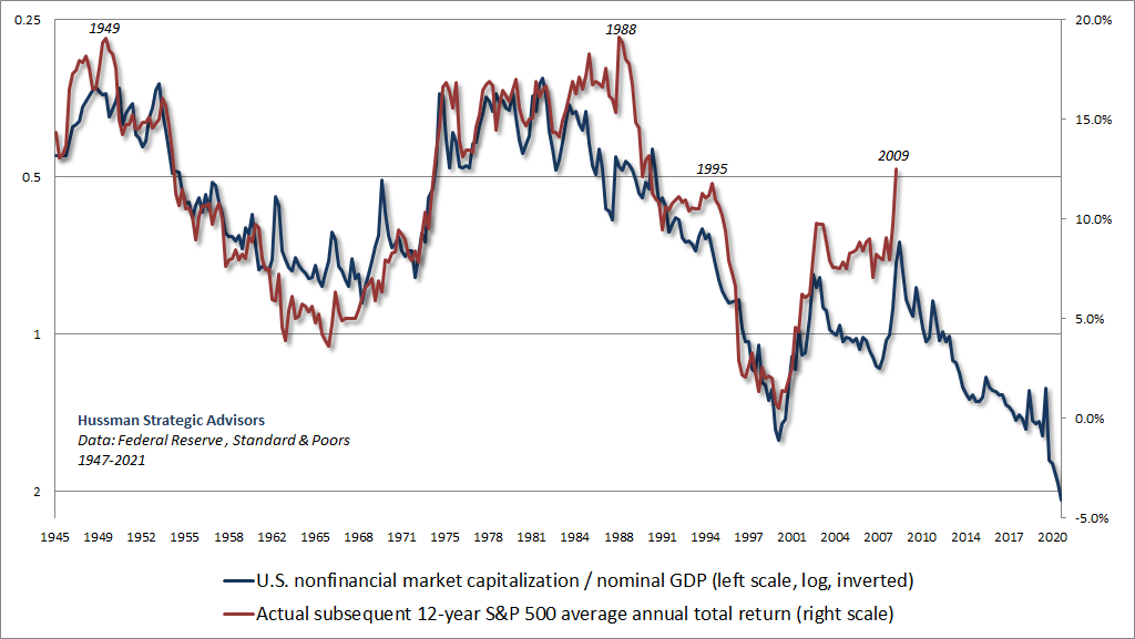
Notice that the 1949 starting period referenced by Graham features one of those “errors.” Why? Subsequent market returns were higher than expected because valuations doubled by the early 1960’s, to levels well above their historical norms. That “error” was subsequently corrected by two decades of market returns that fell far short of prior experience. Another “error” is evident in the 12-year period that followed 1988. Why? Count forward 12 years. 2000 was a bubble peak. The market suffered negative returns for over a decade. Another “error” was evident in the 12-year period that followed 1995. Why? Count forward 12 years. 2007 was the peak of the mortgage bubble, and was followed by a 55% collapse in the S&P 500 during the global financial crisis. Always a reckoning.
In this context, the recent “error” between projected returns and actual market returns isn’t an indication that valuations aren’t “broken.” Rather, this is an example of the same principle that Graham wrote about decades ago, with the same probable outcome. Only the date has changed: Few people are willing to consider seriously the possibility that the high rate of advance in the past means that stock prices are now too high, and hence that the wonderful results since 2009 imply not very good but bad results for the future.
Geek’s Note: I prefer to evaluate the relationship between valuations and returns over a 12-year horizon because that’s the point where the autocorrelation profile of most good valuation measures hits zero, meaning that it’s the most reliable horizon over which mean-reversion occurs. The relationships look nearly identical for 10-year returns, but become much “noisier” as the investment horizon shortens to less than 4-5 years.
I’ve often observed that the denominator of every useful valuation multiple is basically shorthand for the very long-term stream of future cash flows that will be delivered into the hands of investors over time. When a good market valuation measure rises, the extra return you celebrate has simply been removed from the future. When a good market valuation measure collapses, the shortfall of return that you suffer has also been added to the future. It’s important to know where you stand in that cycle.
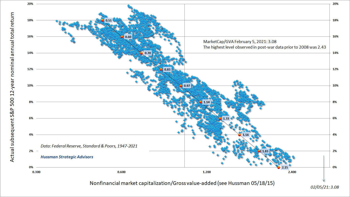
The chart below is reprinted from last month, and shows the relationship between our measure of nonfinancial market capitalization to corporate gross value-added (MarketCap/GVA) and actual subsequent 12-year total returns for the S&P 500, in data since 1950.
For reliable valuation measures, you can prove to yourself that if X is, say, the 12-month total return of the market in excess of the 10-12 year annual return you projected at the beginning of the year, log(1+X) will, or at least should, have a correlation of about -0.9 or better with the change in your 10-12 year projection. That is, a short-term return significantly above your long-term projection should result in a corresponding reduction in that long-term projection. If not, your valuation measure is inconsistent.
When a good market valuation measure rises, the extra return you celebrate has simply been removed from the future. When a good market valuation measure collapses, the shortfall of return that you suffer has also been added to the future. It’s important to know where you stand in that cycle.
As usual, I’ll note that one does not need to “correct” the relationship between valuations and projected returns for the level of interest rates. The belief that such a correction is needed reflects a profound misunderstanding of how asset pricing works, and confusion about the contexts where interest rates become relevant (e.g. choosing a cost of capital in the absence of an observable price). One can certainly compare the estimated return of stocks with the level of interest rates, but price and expected future cash flows are the only objects that one requires in order to estimate future returns.
Extreme leverage, extreme valuations, and liquidation risk
Last month, we observed an interesting canary in the coalmine in the collapse of Archegos Capital, which amassed billions of dollars of wildly leveraged stock positions, using swap market instruments to conceal the extent of its overexposure. One of the more obvious and almost pedestrian measures of investor leverage is the ratio of margin debt to GDP, which has spiked by more than 45% over the past 9 months. It’s certainly not a measure that we’d use in isolation, but amid the most extreme valuations in history, highly leveraged investment positions imply considerable risk of forced, price-insensitive liquidation.
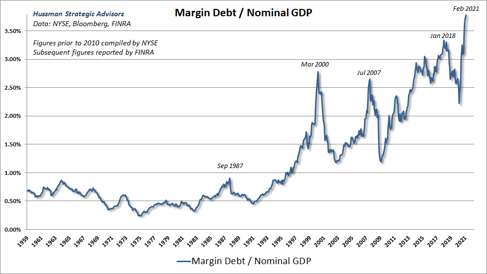
Normalizing margin debt by GDP (rather than, for example, market capitalization) matters, because it captures the valuation effect:
MarginDebt/GDP = MarginDebt/MarketCap * MarketCap/GDP
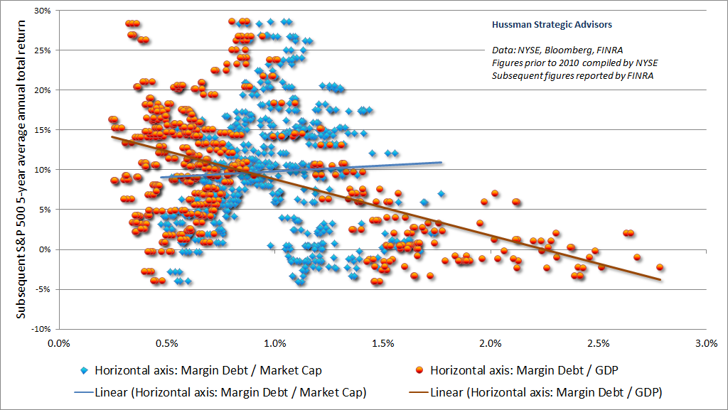
In contrast, normalizing margin debt by market capitalization divides by same object one wants to project, which gives credit to a hypervalued market and destroys the relationship with returns. In fact, there is actually a positive relationship between margin debt/market cap and subsequent 5-year S&P 500 total returns. The chart below shows the difference between these two measures.
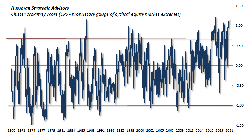
Meanwhile, as I noted last month, we’re seeing an unusual overlap of high-risk conditions that correlate with those that often precede steep market collapses – a collection of measures capturing valuations, internals, sentiment, leverage, overextension, and yield pressures. Below, I’ve presented another one of our internal gauges that incorporates a similarly broad range of measures. It essentially measures the “proximity” of current conditions to clusters associated with either abrupt market losses or steep market gains. Present conditions fall into a fairly extreme subset that includes February 2000, early-October 2018, January 2018, January 2014 (though only followed by a 5% market correction over the following 3 weeks in that instance), October 2007, March 2000, July 1998, August 1987, and December 1972. That’s not the best group of periods to be associated with, and is certainly nowhere close to the opportunities of 2009, 2002, 1990, 1982, 1974, or even lesser but more recent market lows.
All of that said, we have no “target levels” or specific outcomes that need to be reached as a prerequisite to shift to a more neutral or constructive outlook. Even if the S&P 500 was to go nowhere for a decade, it would almost certainly do so in an interesting way, with numerous points where a material retreat in valuations will be joined by an improvement in our measures of market internals. Nothing in our value-conscious, historically-informed, full-cycle investment discipline requires valuations to retreat to historical norms ever again. The risk of a steep plunge on forced liquidation is certainly worth considering, but our current investment outlook is based on observable conditions such as valuations, market internals, yield pressures, and so forth, not on any forecast, projection, or price target.
Relying on psychological discomfort
There can be few fields of human endeavor in which history counts for so little as in the world of finance. Past experience, to the extent that it is part of memory at all, is dismissed as the primitive refuge of those who do not have the insight to appreciate the incredible wonders of the present.
– John Kenneth Galbraith
In every speculative episode, the mere concept of “market history” is viewed with derision.
In that context, it’s useful to remember that whatever wonders one believes have been achieved by technology, the Federal Reserve, or blockchain tokens, a share of stock is still at bottom simply a claim on some future set of cash flows that will be delivered into the hands of investors over time. Overvaluation does not create more “wealth.” The actual wealth is in the stream of cash flows and value-added production that will be created and delivered over time. If a security can be expected to deliver a single $100 payment in the future, driving the price to $200 doesn’t create more “wealth” in the economy. The holder can’t realize “wealth” from the overvalued security without selling it to someone else. Overvaluation simply enables the holder to obtain a transfer of wealth from some poor soul who is willing to buy at that price.
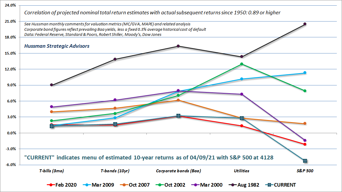
In my view, it’s dangerous to imagine that the low returns available on Treasury bonds haven’t also fully permeated other markets, particularly stocks and corporate debt. There seems to be a popular delusion – an extraordinary madness of the crowd – that even at the most extreme stock market valuations and the lowest corporate bond yields in history, low interest rates leave investors “no alternative” but to chase risk, regardless of the price. Investors seem to imagine that weak investment prospects are a feature of Treasury bonds, but nothing else.
The chart below shows our 10-year projections for various conventional asset classes. Each line is a separate point in time. These include the 1982, 2002, and 2009 market lows, as well as the 2000, 2007, 2020 and current market highs. The current profile of prospective returns across various asset classes looks almost identical to the profile at the 2000 market peak, only substantially lower across the board.
For investors who remain convinced that the Federal Reserve can “save the day” regardless of extreme valuations, they should at least understand how monetary policy operates. Quantitative easing simply means that the Fed buys interest-bearing bonds and replaces them with zero-interest base money (currency and bank reserves). This base money must be held by someone at every moment in time, in the form of base money, until it is retired. If you hold some of that zero-interest base money, you can certainly buy stocks with it, but then you get the stocks and the seller gets the base money. The moment it goes “into” the stock market, it comes “out of” the stock market. Base money just passes from one holder to another like a hot potato.
The pure psychological discomfort of zero returns has produced a stock market that is now priced for negative returns. Unfortunately, investors who rely on zero-interest money to prop up the stock market require a world where everybody ignores valuations; a world where expected stock market returns are always greater than zero, and always worth the risk, regardless of how extreme valuations might be.
Good luck with that. As usual, we’ll continue to align our market outlook with valuations, market internals, and other factors as those conditions change over time. We’re very comfortable with hedged equity here, and with our ability to shift the extent of that hedging. Remember that even though I correctly projected negative 10-year S&P 500 total returns at the 2000 market peak, valuations and market internals improved enough by early-2003 to encourage a constructive outlook. Even though I viewed the market as steeply overvalued in 2007, before the global financial crisis, I observed late-October 2008 that stocks had become undervalued. In late-2017, we adapted our discipline to defer our bearish response to “overvalued, overbought, overbullish” extremes until we see deterioration and divergence in our measures of market internals. We do observe this sort of deterioration at present, but we’ll also defer our bearish outlook if internals improve.
The pure psychological discomfort of zero returns has produced a stock market that is now priced for negative returns. Unfortunately, investors who rely on zero-interest money to prop up the stock market require a world where everybody ignores valuations; a world where expected stock market returns are always greater than zero, and always worth the risk, regardless of how extreme valuations might be.
Following our late-2017 adaptation, we’re content to gauge investor speculation or risk-aversion (largely based on our measures of market internals), without assuming any well-defined “limit” to either. I expect that we can comfortably navigate whatever sort of extreme or misguided policy we might encounter, without abandoning our attention to valuations or market internals, and without blindly surrendering every bit of intellect to the idea that “this time is different.” I remain convinced that a value-conscious, historically-informed, full-cycle discipline is preferable to resting one’s future on the belief that the psychological discomfort of zero-interest money will magically and permanently make everything ok.
The extent of the market’s shrinkage in 1969-70 should have served to dispel an illusion that had been gaining ground during the past two decades. This was that leading common stocks could be bought at any time and at any price, with the assurance not only of ultimate profit but also that any intervening loss would soon be recouped by a renewed advance of the market to new high levels. That was too good to be true.
– Benjamin Graham, The Intelligent Investor
Public health note
Since the beginning of 2020 when the first few cases of SARS-CoV-2 infection were identified in the U.S., I’ve been engaged with researchers, public health officials, and legislators on the response to the COVID-19 pandemic, as part of the efforts of the Hussman Foundation. Among the most distressing aspects of the pandemic has been its brutally unforgiving arithmetic. Only two barriers stand in the way of a highly infective virus ripping through a population: 1) the percentage of the population that remains susceptible (which declines as a result of past infection or vaccination) and; 2) the extent to which containment behaviors reduce interactions that would otherwise lead to infection (distancing, smaller groups, face coverings – especially in indoor settings involving conversation or expelled air, avoiding superspreader events, and so forth).
For any new case of infection, the average number of additional people who go on to be infected is called the “reproductive rate.” If everyone is susceptible, that number is called the “base” reproductive rate R0. The fraction of the population still at risk declines as people acquire immunity or vaccination. So gradually, each interaction has a lower probability of infecting a susceptible person. Containment behaviors further reduce the number of subsequent infections. The reproductive rate at time t is simply called Rt.
In the adapted SIR (susceptible, infected, recovered) model that I developed at the Hussman Foundation, this gives us a very simple way to think about the average number of new infections at any time t after the virus first appears:
Rt = R0*s*c
where R0 is the base reproductive rate, s is the susceptible share of the population {0,1}, and c is the “tightness” of containment measures, also {0,1} where 1 is no effort and 0 is full isolation. Those two little variables affect whether the trajectory of the pandemic is mild or utterly brutal.
For the original variant of SARS-CoV-2, the most common estimate for R0 is about 2.6 (our own estimate is slightly lower, at about 2.4). By late-January 2021, we could estimate based on numerous relationships that the susceptible share of the population had gradually declined to about 0.7. Meanwhile, our estimate of containment tightness in January 2021 was about 0.5 (a figure that hasn’t changed since early November).
So in late-January, with Rt = 2.6*0.7*0.5 = 0.91, we saw a sharp drop in the pandemic trajectory, at least for the original SARS-CoV-2 variant.
A value of Rt below 1.0 is what defines “herd immunity” – it’s not where spread drops to zero, but is instead where the spread stops being exponential, so that local containment efforts have a chance of stopping any new outbreaks. Importantly, the drop we’ve seen since late-January doesn’t reflect true herd immunity. Rather, it wholly relies on continued containment behaviors. It’s what I call “synthetic” herd immunity.
As a counterfactual, had we dropped containment efforts in January, c would have jumped to 1.0 and Rt would have jumped to 2.6*0.7*1.0 = 1.82, allowing the virus to continue ripping through the population.
Unfortunately, that’s exactly what novel variants were already doing. Near the end of October 2020, novel variants of the SARS-CoV-2 virus began circulating in the United States. The main adaptation of these variants involves changes to the “receptor binding domain,” which allows the virus to attach more strongly to respiratory cells, and by some reports, to multiply more rapidly in the lower respiratory tract. These variants are estimated to be about 50% more infective than the original variant of the virus.
So now multiply R0 by 1.5 and do the same math. As of late January, even as the original variant was constrained at least by “synthetic” herd immunity, the novel variants still had Rt = 1.5*2.6*0.7*0.5 = 1.37. As a result, the novel variants continued to expand, even though the original variant was in retreat. That’s why continued containment efforts have been so essential, at least until we get the vaccinated percentage of the population high enough to enable herd immunity through reductions in population susceptibility (s) alone.
Fortunately, the effectiveness of the vaccine rollout in the U.S. has been remarkable. As a result of past infection, coupled with vaccination, I currently estimate that only about 49% of the U.S. population remains susceptible to SARS-CoV-2 infection, with a disproportionate share of older, more vulnerable people vaccinated – to the point where I estimate that the fatality rate in the event of infection has likely declined by at least 35%. By the way, while all of these estimates seem very casual, there’s a whole database of information, studies, and calculations behind them.
Let’s do the math again for the new variants, given 1.5x infectivity, continued containment effort at c = 0.5, but with s down to 0.49: Rt = 1.5*2.6*0.49*0.5 = 0.96.
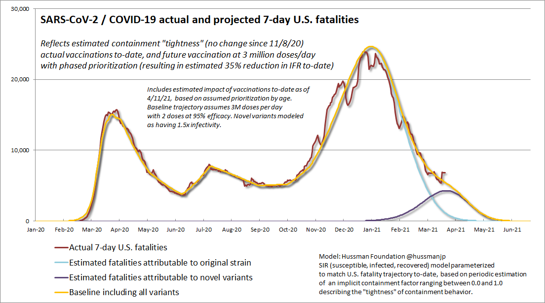
With that, I believe that we’ve also just reached “synthetic” herd immunity with respect to the novel variants, provided that we sustain containment behavior. Even better, assuming that the U.S. vaccination rate continues at 3 million or more doses per day, only about 10 more weeks of diligent containment efforts will be needed. At that point, the pandemic will be essentially over, at least in the U.S., though tragically not for many other countries (where U.S. leadership and assistance is really essential). Again, we are not currently at the point where infections will stop. Indeed, herd immunity actually occurs where novel infections are near their highest point. Also, because we’ve only reached “synthetic” herd immunity at the moment, it’s also heavily dependent on continued containment effort for a bit longer. Still, we’re getting close to the finish line, and the trajectory is very hopeful in any case.
The chart below shows our estimate for U.S. 7-day COVID-19 fatalities. You’ll note that there are actually two separate curves that define this trajectory. One is for the original variant, and the other is for the novel variants. The overall trajectory is just the sum of the two. There’s a little pop in the most recent data, I suspect related to Easter travel, but hopefully it doesn’t reflect any significant relaxation in containment behavior. As we’ll see below, the combination of sustained containment practices and a high vaccination rate has helped to prevent what would have otherwise been a disastrous curve for the novel variants.
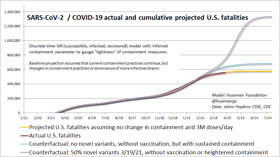
Given the remarkable and unfortunately devastating accuracy of this pandemic arithmetic, it’s possible to estimate “counterfactuals” – that is, outcomes that might otherwise have occurred if certain factors (containment practices, vaccination, novel variants) had been different.
The chart below shows what the trajectory of cumulative U.S. fatalities would have looked like depending on the presence or absence of novel variants, and on vaccination rates. The worst outcome, by far, is the trajectory we would observe simply by setting vaccination figures to zero. That’s literally the only difference between the highest trajectory and the current one. We would look like Brazil.
Undoubtedly, the U.S. would have responded to the “no vaccination” trajectory with fresh lockdown measures, so I doubt that it would have been allowed to become so devastating. But that’s exactly the point – it’s the success we’ve had in vaccination rates that has prevented what would otherwise been almost certain fatalities, lockdowns and economic disruptions. In my view, that’s an enormous accomplishment.
A final note, for those familiar with my scientific research (most of my published papers focus on cellular and molecular pathways of complex disease). I’ve been fairly open in my concerns with showing the viral receptor binding domain (RBD) to our immune system in the full Monty. It’s very “tasty” and immunogenic, so it gets a lot of its attention, but it’s also highly susceptible to mutation and can provoke certain maladaptive immune responses. That certainly weakens the effectiveness of natural infection in protecting against future strains, and I do wince at the possibility of future variants coming in contact with anti-spike RBD antibodies that don’t neutralize the virus and contribute to immune-enhanced disease instead.
It’s exactly for that reason that I’ve been enormously encouraged (there was jumping involved) by the fact that the vaccines approved in the U.S. have all been designs that stabilize the spike in a “pre-fusion” conformation that broadens the antibody response to parts of the spike that are “conserved” across different variants, and limits presentation of the RBD. I do believe that any vaccine is better than none, particularly at this point in the pandemic, but I do prefer these designs. I’m happy to note that I’ve got at least one family member who has been vaccinated by each of the three vaccines with an EUA in the U.S. (Pfizer, Moderna, Johnson & Johnson), and I’m very comfortable with all of them.
Keep Me Informed
Please enter your email address to be notified of new content, including market commentary and special updates.
Thank you for your interest in the Hussman Funds.
100% Spam-free. No list sharing. No solicitations. Opt-out anytime with one click.
By submitting this form, you consent to receive news and commentary, at no cost, from Hussman Strategic Advisors, News & Commentary, Cincinnati OH, 45246. https://www.hussmanfunds.com. You can revoke your consent to receive emails at any time by clicking the unsubscribe link at the bottom of every email. Emails are serviced by Constant Contact.
The foregoing comments represent the general investment analysis and economic views of the Advisor, and are provided solely for the purpose of information, instruction and discourse.
Prospectuses for the Hussman Strategic Growth Fund, the Hussman Strategic Total Return Fund, the Hussman Strategic International Fund, and the Hussman Strategic Allocation Fund, as well as Fund reports and other information, are available by clicking “The Funds” menu button from any page of this website.
Estimates of prospective return and risk for equities, bonds, and other financial markets are forward-looking statements based the analysis and reasonable beliefs of Hussman Strategic Advisors. They are not a guarantee of future performance, and are not indicative of the prospective returns of any of the Hussman Funds. Actual returns may differ substantially from the estimates provided. Estimates of prospective long-term returns for the S&P 500 reflect our standard valuation methodology, focusing on the relationship between current market prices and earnings, dividends and other fundamentals, adjusted for variability over the economic cycle.