

Alice’s Adventures in Equilibrium


John P. Hussman, Ph.D.
President, Hussman Investment Trust
June 2021
I daresay you haven’t had much practice. Why, sometimes I’ve believed as many as six impossible things before breakfast.
– The Queen, Alice’s Adventures in Wonderland, Lewis Carroll
Coherent thinking is interested in how things are related; where they come from, where they go, and the mechanisms by which they affect each other. Incoherent thinking is a world of magic, loose theory, and superstition; where things pop into existence, vanish without a trace, and are somehow related without any need to carefully describe cause and effect.
Much of what passes for economic and financial analysis is incoherent. I’ve chosen that word carefully. The problem is not that the beliefs of investors are “less true” than they think. It’s that many of the most commonly repeated phrases don’t mean anything close to what investors think they mean. It’s that many of these belief systems are inconsistent, confused, or rooted in false premises. They are incoherent in the same way that it’s incoherent to debate how many pine trees are planted at the edge of the earth, how many aardvarks you need to start a thunderstorm, or how the gold coins in the pot at the end of the rainbow are invested.
That’s not to say that incoherent beliefs have no impact on the markets. But it does mean that the speculative market impact is entirely the product of what Buddhists might call “mental formations” that may not, and need not, have anything to do with reality, and leave investors vulnerable because of it.
Equilibrium is like conservation of mass
The most frequent way that investors come to believe in impossible things is that they fail to impose “equilibrium.” They neglect to examine how output and securities come into existence, the arithmetic that dictates how they have to add up, and who ends up with what after each exchange. They imagine that what might be true for an individual investor or sector must also be true for the financial markets or the economy as a whole.
Discussions of economics and finance typically reflect little consideration or even understanding of the “stock-flow equilibrium” that necessarily relates various real economic outcomes – output, savings, investment, and government spending – with the issuance of various financial objects like Treasury debt, base money, and stock shares. Equilibrium is like conservation of mass – every purchase is also a sale; every security that’s created must be held by someone until it is retired; securities are created to memorialize obligations; output that’s not consumed has been saved; the shortfall of one sector must be the surplus of another. Once you insist on thinking in terms of equilibrium, it becomes obvious how many discussions in economics and finance are incoherent.
Notably, the lack of equilibrium thinking obscures a critical fact about investing: every security, once issued, must be held by someone until it is retired. As a result, the only thing that a security will ever provide to its investors, in aggregate, is the stream of actual cash flows that it delivers between the point that it is issued and the point that it is retired. The price changes called out by Mr. Market are not changes in aggregate wealth – they mainly provide varying opportunities for wealth transfer between one investor and another. There’s an increase in aggregate wealth only if there’s an increase in expected value-added output and deliverable cash flows. Otherwise, a change in the valuation of a given stream of cash flows merely reflects a change in the expected rate of return.
Imagine that in some private business you own a small share that cost you $1,000. One of your partners, named Mr. Market, is very obliging indeed. Every day he tells you what he thinks your interest is worth and furthermore offers either to buy you out or sell you an additional interest on that basis. Sometimes his idea of value appears plausible and justified by business developments and prospects as you know them. Often, on the other hand, Mr. Market lets his enthusiasm or fears run away with him, and the value he proposes seems to you a little short of silly. You may be happy to sell out to him when he quotes you a ridiculously high price, and equally happy to buy from him when his price is low. But the rest of the time you will be wiser to form your own ideas of the value of your holdings, based on full reports from the company about its operation and financial position.
– Benjamin Graham, The Intelligent Investor
We’ll begin with an overview of market conditions, and move on to a discussion of securities, wealth, money creation, fiscal policy, inflation, the Phillips Curve, Bitcoin, market valuations, free enterprise, natural monopoly, and economic growth. I’ve briefly included several charts and points that are familiar to long-time readers – more detail can be found in prior commentaries. My hope is that by the end of this comment, you’ll have a more coherent sense of how they all interact. Ideally, this comment will serve as something of a reference – if only so future investors might avoid the sort of misperception that has contributed to the current extremes.
Market conditions
I’ll note at the outset that understanding how the relationships between money, finance, and the economy actually work may not help your investment process unless you also accept (as we finally did in late-2017) the extent to which the discomfort of investors with zero interest rates has blunted their capacity for discernment. Amid zero interest rates, historically reliable “limits” to speculation have not applied.
That’s not to say that the current speculative extremes will escape profoundly damaging consequences. It’s just that we have to be selective in our disdain. In particular, we have to be content to gauge the presence or absence of speculation or risk-aversion, without assuming that there is a limit to either.
When investors form their expectations for returns based on price behavior, and price behavior is driven by investor expectations in turn, the feedback loop contributes to self-reinforcing bubbles. The situation is worse when investors ignore valuations in hopes of limitless “support” from policy makers, despite the absence of any reliable, mechanistic relationship – other than psychology itself – linking policy actions and security prices.
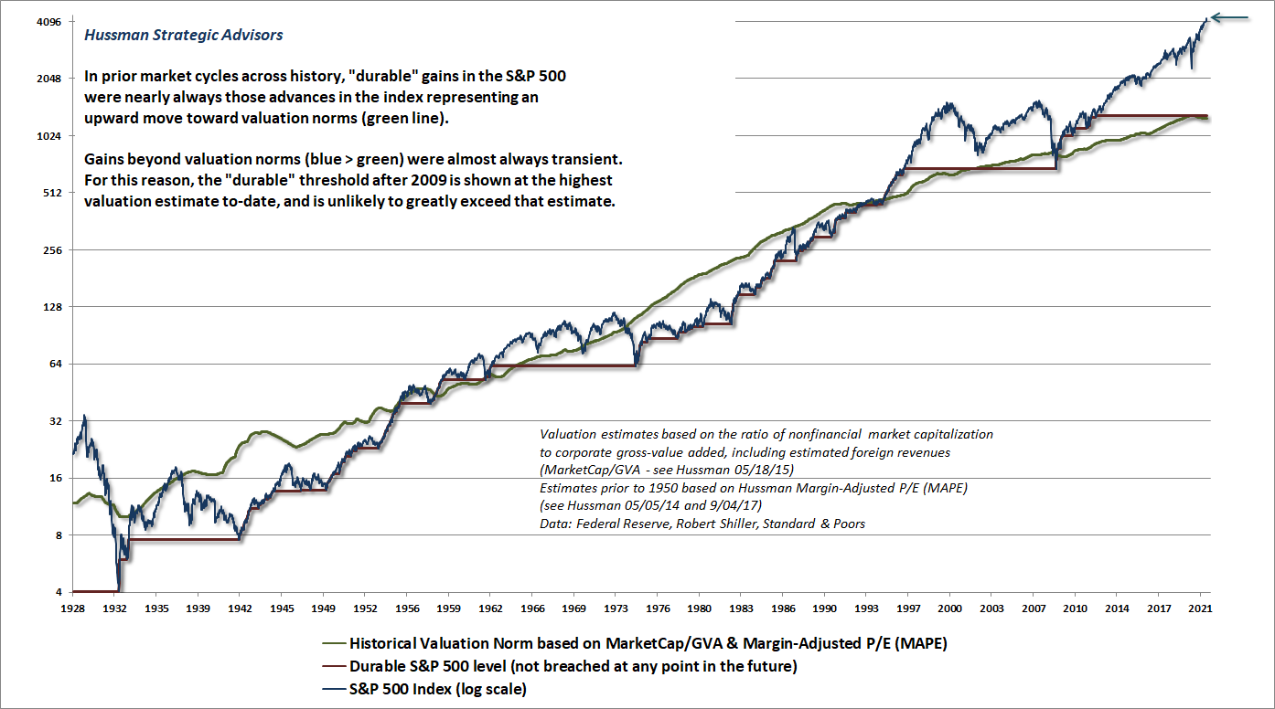
The chart below shows the ratio of nonfinancial market capitalization to corporate gross value-added, including estimated foreign revenues. This is the valuation measure that we find best-correlated with actual subsequent market returns across a century of market cycles, as well as in recent decades.
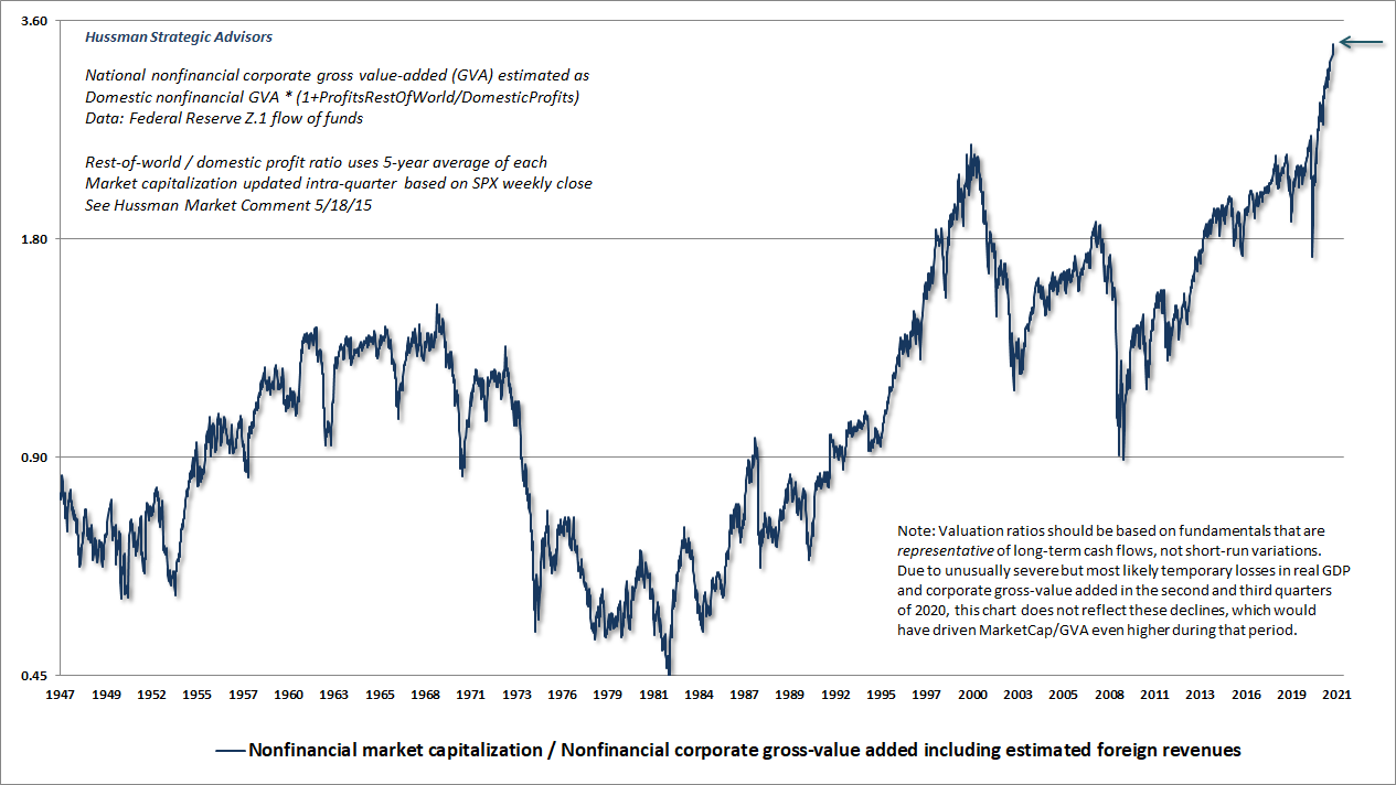
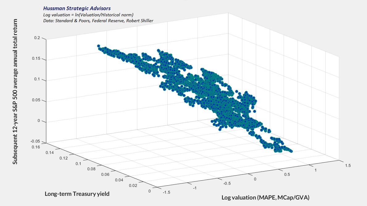
Presently, we estimate clearly negative average annual total returns for the S&P 500 over the coming 12-year period. The scatter below reflects two of our most reliable valuation measures: nonfinancial market capitalization to corporate gross value-added (including estimated foreign revenues) in data since 1950. I’ve extended the chart back to 1928 by setting valuations in proportion to our margin-adjusted P/E (MAPE) in data prior to 1950. The valuation of the U.S. stock market on June 11, 2021 was easily the highest level in history.
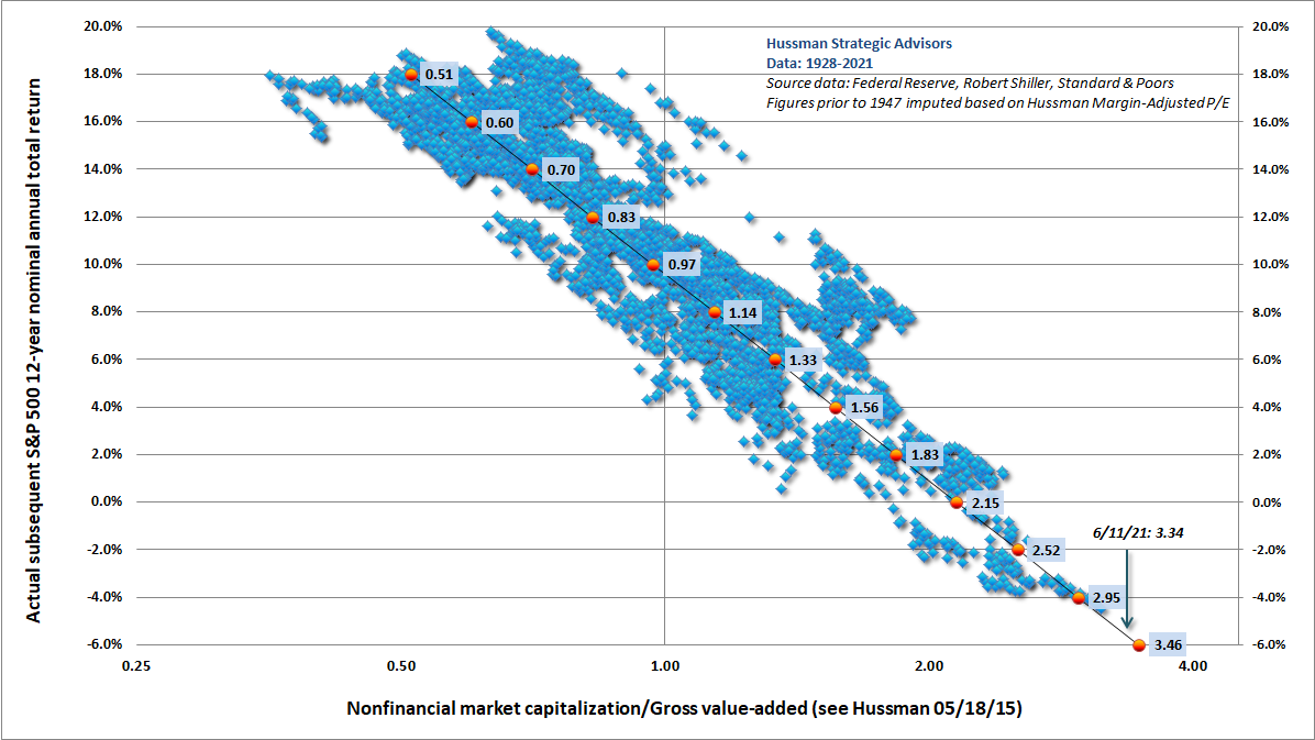
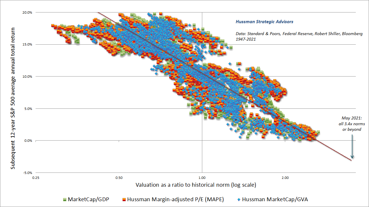
The scatter below reflects data since 1947, showing our Margin-Adjusted P/E (MAPE), MarketCap/GDP and MarketCap/GVA versus actual subsequent 12-year S&P 500 total returns. These are among the valuation measures we find best-correlated with actual subsequent market returns. Notice that each is normalized so that 1.0 on the horizontal axis represents the historical norm. Not surprisingly, when valuations have been near their historical norms, subsequent returns have averaged something close to 10% annually. That’s what we mean when we discuss the “mapping” between valuations and subsequent returns.
What drives “errors” in this mapping? Errors are produced mainly when valuations at the end of a given holding period are very far from their historical norm, at least temporarily. For example, if current valuation extremes were sustained at these levels even 12 years from today, the average annual total return of the S&P 500 over that period would likely be in the low single digits, rather than the negative return that we presently expect. That low, but positive return would quite likely be associated with substantial interim volatility, because extreme valuations are typically followed by high volatility, as prices become more sensitive to small changes in expected returns. Still, we can’t rule out future bubbles, so even at current extremes, we have to navigate and respond to market conditions as they change.
It’s important to recognize that while valuations are extremely informative about prospective market returns on a 10-12 year horizon, and potential market losses over the completion of any market cycle, valuations are not reliable short-term measures. If elevated valuations were enough to drive the market lower, we could never observe the sort of extremes that emerged in 1929, 2000 and today. Over shorter horizons, we have to attend to whether investors are inclined toward speculation or risk-aversion, and we find that this psychology is best gauged by the uniformity or divergence of market internals across thousands of individual stocks, industries, sectors, and security-types, including debt securities of varying creditworthiness.
Presently, our key gauge of market internals is also unfavorable, while market conditions are extremely overextended, which creates the potential for “trap door” outcomes. We’ve seen this combination a few times in recent years, particularly in the fourth quarter of 2018 and the first quarter of 2020. Based on statistical proximity, we find that the “nearest neighbors” to current extremes were in 1987 and 1998, just before “panic” type declines, neither which was accompanied by a recession. Even amid these extremes, we’ve patiently refrained from “fighting” this speculation aggressively until we observe broader deterioration in the equity components of internals. For now, the main divergences on the equity side take the form of progressively weaker participation, leadership, and price-volume behavior with each successive market advance.
While Wall Street is clearly enthusiastic about an enormous post-pandemic recovery, keep in mind that the U.S. government has run a deficit amounting to about 19% of GDP over the past year. Undoubtedly, we’ll see a broad recovery in private sector economic activity in the quarters ahead. But this recovery will also have to replace, rather than augment, trillions of dollars in pandemic relief funds. The recovery will progress amid substantial labor market frictions as well as shortages in various production inputs. It’s quite possible that the mental image in anticipation of a post-pandemic recovery may be more pleasant than the actual recovery itself. In that event, the glowing optimism currently built into record valuation extremes could be followed by quite a bit of disappointment.
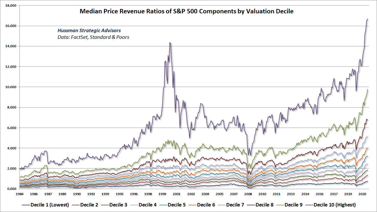
This is not a market that is priced for the smallest shred of disappointment. Below, we’ve sorted S&P 500 into 10 deciles, by price/revenue ratio (thanks as usual to our resident math guru Russell Jackson for compiling all of this data). Each line shows the median price/revenue ratio of each decile. Keep in mind that the lowest valuation deciles typically represent companies in industries such as retail and industrials, while the highest valuation deciles typically represent companies in industries like information technology and medical devices. So each line is best compared with its own history. Presently, every one of these deciles is at the most extreme level in history (unlike the 2000 peak, when there was far more dispersion across valuations). This is breathtaking, and I don’t expect it to end well.
Still, even here, we can’t assume that speculative recklessness has a well-defined limit. An improvement in our gauge of market internals, either at current valuation levels, or ideally at lower ones, would encourage a more neutral outlook (though certainly with a safety net in any event). That would not relieve the dismal long-term prospects for stocks – I expect this bubble to collapse like every bubble that has preceded it. Still, if one adaptation has been necessary in the face of zero interest rate policies, it’s that speculation should not be aggressively fought with an outright bearish outlook except when growing dispersion and divergence in market action suggests that the “bit” has dropped out of investors’ teeth. We’ll take that evidence as it emerges.
As a side note, it’s endlessly fascinating to me that investors imagine that decades of zero interest rate policies by the Bank of Japan have somehow held stocks at a “permanently high plateau.” As an advisor to the Bank of Japan, my late friend and dissertation advisor Ronald McKinnon at Stanford argued – even 30 years ago – against the sort of “financial repression” it was pursuing. Ben Bernanke encouraged the opposite.
In the span of more than 30 years since the December 1989 speculative peak, Japan’s real GDP growth has averaged less than 1% annually. Meanwhile, the Nikkei has produced a total return of zero, but not without three separate losses exceeding 60% each, four distinct additional declines in the 30-40% range, and multiple smaller corrections closer to 15-20%.
This sort of market outcome is what I’ve often described as a “long, interesting trip to nowhere.” Such periods invariably follow of record valuation extremes. Recall, for example, that the total return of the S&P 500 lagged Treasury bills during the 18-year period from August 1929 to May 1947, and during the 21-year period from November 1961 to October 1982, and during the 13-year period from March 2000 to April 2013. That’s 52 years out of an 84-year span. It’s just what happens when valuations become extreme.
In my view, much of the cartoonish behavior that we observe in various markets and asset classes is directly or indirectly Fed-induced. Explosive growth of monetary hot potatoes, coupled with years of zero-interest rates, have fueled an increasingly reckless speculative appetite for alternatives that might escape (or profit from) the Fed’s unrestrained activism and financial repression. If we insist on Japan-style monetary dogma, we should be fully prepared for Japan-style outcomes.
Every security that is issued must be held by someone until it is retired
Consider a world where Alice has $100 of what people call “cash on the sidelines,” and Becky owns some stock certificates in ABC. It seems obvious that Alice can take her “cash on the sidelines” and instead put her cash “into the stock market” by buying 10 shares of ABC stock from Becky at $10 each. These phrases like “cash on the sidelines” and “moving cash into the stock market” all make sense, as long as we ignore Becky. Unfortunately, the moment we think about Becky, it’s clear that both phrases are completely incoherent.
Who holds the cash now? Becky. It hasn’t somehow moved “off the sidelines.” Who holds the stock now? Alice. All that has happened is that the owners have changed. In equilibrium, there are no “sidelines.” The stock market isn’t some big jar on Wall Street where money “flows” in. Every security that is issued, whether it’s base money (currency and bank reserves), or stock shares, or bond certificates, must be held by someone, exactly in the form it was issued, until it is retired.
What if Alice buys stock in an initial public offering? Let’s work it out. Alice transfers her $100 of cash to Charlie, who has started ABC – his own business. Charlie issues 10 shares to Alice at $10 each. Those new shares are evidence that money has been “intermediated” from Alice to Charlie, and in return, Charlie now owes Alice a portion of the cash flows from his business. Where did the cash go? Charlie has it. It didn’t disappear. Somebody has to hold the cash until it is retired. The new stock shares memorialize the transaction: they are an asset to Alice, and a liability to Charlie.
What if Charlie puts the $100 of cash in the bank? Well, now Charlie’s bank creates a security, called a “deposit” to memorialize the exchange of funds. The deposit is an asset to Charlie, and a liability to Charlie’s bank. The bank now holds $100 of bank reserves as an asset that “backs” Charlie’s deposit. There is no more base money than there was before. No net wealth has been created. There’s just a new deposit asset, which is also a new deposit liability.
What if Charlie’s bank lends the $100 of reserves to Deena? Well, a new security is created, called a “loan certificate” to memorialize the exchange of funds. The loan is an asset of the bank (which now “backs” Charlie’s deposit instead of bank reserves), and a liability to Deena. Deena might take the $100 of base money as cash, or she might deposit in the bank like Charlie did. Has the creation of the loan or the deposit created new “wealth” or added to economic output? No. There’s just a new security, or possibly several (depending on how many times the funds are intermediated), each that represents an asset to one person in the economy and a liability to another.
What about price appreciation? What if Deena takes the $100 she borrowed and buys 4 shares of ABC stock from Alice, but now for $25 each? Alice gets back her original $100, she still has 6 shares of ABC, and the market capitalization of ABC has increased. Isn’t there more total “wealth” in the economy because the price of ABC stock went up? Not unless the expected future value-added output and associated cash flows of ABC have also increased, and that’s economic “wealth” that will need to be realized in the future. If the higher price merely reflects an increase in valuations, there’s no increase in current or future economic “wealth” at all. In that case, all that’s happened is the future long-term returns on ABC stock have declined.
Yes, having bought low and sold high, Alice is particularly better off, but only because her transactions have allowed her to obtain a transfer of wealth from other people in the economy.
While the market capitalization of ABC is higher, how does a holder get at it? All of the shares have to be held by someone until they’re retired. Alice and Deena can certainly sell the stock they own for a higher price than before, but only by obtaining a transfer of funds from some new buyer. The true “wealth” embodied in ABC stock is still the stream of future value-added production and the resulting deliverable cash flows that ABC will distribute to its shareholders over time.
Starting to get a feel for this? Securities are not “net” wealth for the economy as a whole. They are evidence that funds have been intermediated from one person in the economy to another. Each one is an asset to some holder and a liability to some issuer. From an individual perspective, every person who owns a financial security may count that asset as personal “wealth,” but it’s really a claim on future cash flows that will be delivered by the issuer. Aside from whatever cash flows the security delivers while one owns it, the only way to realize the “wealth” at any point before the security is retired is to sell it to someone else.
Telescope that into the future and you’ll discover that the “wealth” embodied by any security is simply the stream of cash flows that it will deliver to its holders between today and the point that the security is retired. If new value-added output and income are not produced along the way, those cash flows are just transfers of existing funds from the issuer to the holder. Ultimately, the only thing that creates new net wealth for the economy as a whole is value-added output that is produced but not consumed. Everything else is price fluctuation and wealth transfer between individuals.
Suppose Elwood builds a bench from a tree in his backyard. Assume it’s durable enough to be considered housing “investment” rather than consumption. If Fiona wants to purchase it but doesn’t have the assets, Fiona can give an IOU to Elwood. One person in the economy has produced something, someone else has purchased it, and in the absence of other funds to transfer, a new debt security has been created to memorialize the exchange. If you net out all the new things in the economy, you’ve got the bench – the saved value-added output. Yes, there’s a new debt security, but it’s not aggregate wealth. It’s simultaneously an asset to Elwood and a liability to Fiona, and it nets to zero. The security just tells you which direction future cash flows have to go between two people in the economy in order to retire that security.
When one nets out all the assets and liabilities in the economy, the only thing left – the true basis of a society’s net worth – is the stock of real investment that it has accumulated as a result of prior saving, and its unused endowment of resources. Everything else cancels out because every security represents an asset of the holder and a liability of the issuer. Conceptualizing ‘saved or unconsumed resources’ as broadly as possible, the wealth of a nation consists of its stock of real private investment (e.g. housing, capital goods factories), real public investment (e.g. infrastructure), intangible intellectual capital (e.g. education, inventions, organizational knowledge and systems), and its endowment of basic resources such as land, energy, and water. In an open economy, one would include the net claims on foreigners (negative, in the U.S. case). Understand that securities are not economic wealth. They are a claim of one party in the economy – by virtue of past saving – on the future output produced by others.
– John P. Hussman, Ph.D. (2015)
The “money” created by banks is not net wealth
It’s often said that banks “print money out of thin air.” This is also incoherent. Banks simply intermediate funds, creating various objects (mainly “loans” and “deposits”) in the process. These objects memorialize the exchange of funds, but each of these objects is someone’s asset and someone’s liability, and in aggregate, they all net out to zero.
There’s a very strong tendency among investors to count every bank deposit as if it represents “money waiting to be spent” and “cash that has to go somewhere.” That’s not how this works. The moment the Federal Reserve buys a Treasury security from someone, you know that there will be additional base money (currency and reserves) in the economy. But the base money is going to stick around until the Fed removes it. Somebody’s got to hold it.
Economic policies change economic outcomes only if they ease a constraint that was previously binding, or impose a constraint that wasn’t there before. If we’ve learned anything over the past decade, it’s that neither spending nor bank loans are stimulated by new base money once the economy is already drowning in it. Everything you ever learned about “money multipliers” quietly assumes that desirable opportunities are endlessly available; that the quantity of lendable reserves is the only constraint. As a former economics and finance professor, I’m almost embarrassed that our profession teaches such nonsense to students.
The only thing that has been reliably stimulated by quantitative easing (and even then, only in periods where investors have been inclined to speculate), is a yield-seeking game of hot-potato that has driven market valuations to extremes that now imply negative returns in the S&P 500 for more than a decade.
Charlie deposits $100 into his bank account. Charlie’s bank now holds base money, which “backs” Charlie’s deposit. If Charlie’s bank lends the base money to Deena, the bank now has an IOU as an asset which now “backs” Charlie’s deposit, and Deena has an IOU as a liability. Meanwhile, $100 of base money travels to Deena’s bank. Deena has a bank deposit that she counts as an asset. The bank deposit is a liability to Deena’s bank, and Deena’s bank counts the $100 in base money as an asset.
There’s no more base money than there was before. There are, of course, more deposits in the banking system that are counted as “M1,” but beyond $100 of base money that has gone from bank to bank, every bit of so-called “money” creation here is simply a set of offsetting assets and liabilities that net to zero. Emphatically, the M1 “created” by the banking system is not aggregate “wealth.” No money has been “pumped into the economy.” Nothing has been “created out of thin air.” Existing funds have been intermediated. That’s it. Indeed, the only way for any of the lending to actually contribute to new “wealth” is for someone to engage in real economic activity that draws new value-added output into existence.
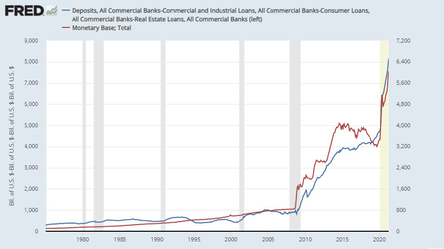
If you look at total deposits in the U.S. banking system, you’ve got some deposits that are “backed” by base money, and others that are backed by “loans” (assets to the bank, liabilities to the borrowers). There’s not an exact relationship between deposits, loans, and base money, because banks can use their assets for investments other than loans, and can fund those investments with other sources than deposits. Still, since bank deposits are primarily backed either by loans or by base money, we find that bank deposits move roughly in line with base money + loans.
The moment the Fed buys Treasury securities and pays for them by creating base money, you’ve got a pretty good indication that bank deposits are going to increase relative to bank loans. But that doesn’t drive people to alter their savings plans, or to run out and spend those deposits. People don’t spend their savings simply because they are holding their savings in a different form. People spend because it serves a need or advances a goal. Quantitative easing doesn’t change that.
Since bank deposits move roughly in line with what “backs” them (base money + loans) it’s no surprise that deposits – loans move hand in hand with the quantity of base money. This is another way of saying that the mountain of bank deposits that people interminably refer to as “cash on the sidelines” is there precisely because the Fed put it there.
What about loans? Hasn’t all the “liquidity” provided by the Fed driven strong bank lending and massive deposit growth via the “money multiplier”?
No.
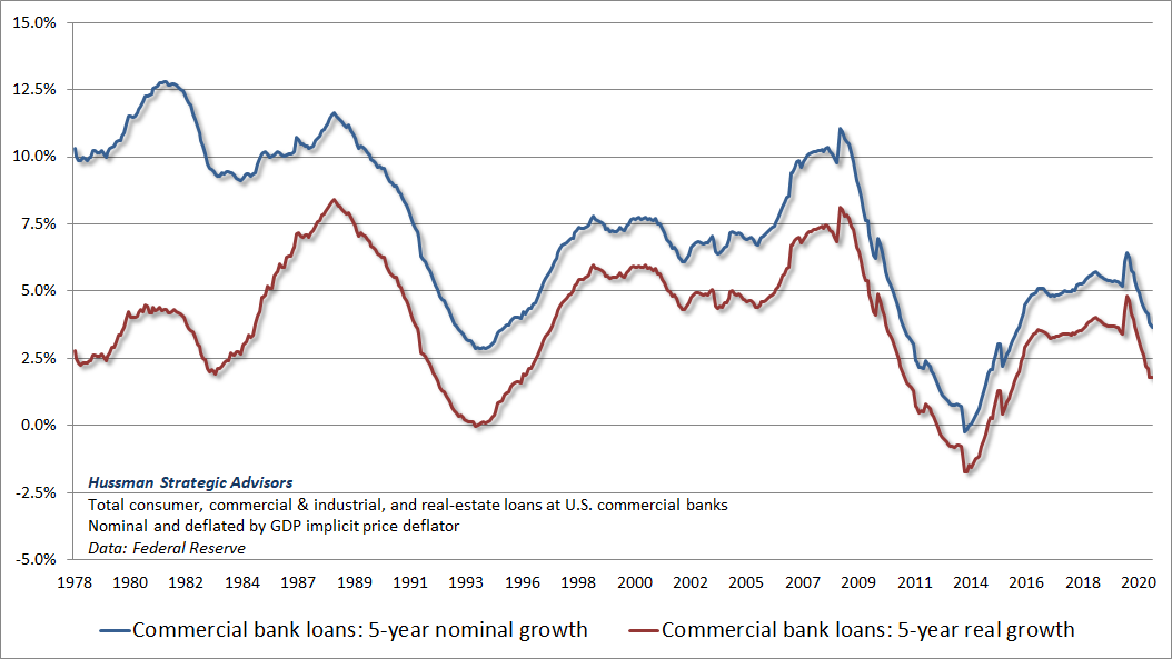
See, here’s the thing. Despite over a decade of deranged Federal Reserve policy – I use that word intentionally to mean both “wildly outside of the historical range” and “bat$%!# crazy” – bank loan growth has been utterly unremarkable. So the growth we’ve seen in bank deposits primarily reflects the fact that the Fed has replaced trillions of dollars of Treasury bills with base money. That’s really the crowning accomplishment of QE – creating a massive pool of zero-interest hot potatoes that someone has to hold at every moment in time, and that does virtually nothing but destabilize the financial system with yield-seeking speculation. The chart below shows 5-year commercial bank loan growth.
Commentators on financial television may gurgle about all the “cash on the sidelines” and speculate why it needs to “flow somewhere,” but these phrases are incoherent. It’s not there because lending has increased, or because “wealth” has increased, or because it’s “waiting to be spent.” It’s there precisely because the Fed replaced Treasury securities with base money that somebody has to hold at every moment in time. It doesn’t need to “flow” anywhere. It’s already there.
Banks are welcome to make more loans, but they do so only if there are creditworthy uses for the funds that the banks are willing to approve. Even then, every loan is both an asset and a liability. You can call these loans “money creation” if you like, but they are not new “savings” and they are not new “wealth.”
Individual depositors can try to get rid of their base money by purchasing stocks (provided that they are inclined to speculate), but the base money just goes to the seller. That’s how we find ourselves amid the most extreme financial bubble in U.S. history. Yet even changes in stock prices aren’t changes in aggregate wealth. The wealth is in the future cash flows, and the value-added production that generates them.
Whatever people choose to do with their deposits, the bottom line is the same. None of this “cash on the sidelines” is going to go away until the Fed removes it. The growth in bank deposits over the past decade has been a nearly mechanical response to the growth in base money that somebody has to hold, at every moment of time. Meanwhile, by encouraging years of yield-seeking speculation, the Fed has done enormous damage, in my view, to the long-term stability of the financial markets. We’ve adapted our discipline in a way that can navigate their speculative effects without embracing their premises, but I continue to have little doubt that it will all end in tears.
Replacing Treasury securities with base money may make savings more ‘liquid,’ but it doesn’t suddenly make people abandon their retirement plans in favor of consuming today. Overvaluation doesn’t create wealth either. It simply enables a wealth transfer from others, and only then if a holder actually sells at the elevated price.
Policy makers sometimes flatter themselves with the idea that holding interest rates at untenably low levels makes it cheaper for borrowers to obtain funds. Unfortunately, it does so only by transferring income from people who are trying to save for the future. Replacing Treasury securities with base money may make savings more “liquid,” but it doesn’t suddenly make people abandon their retirement plans in favor of consuming today. Low rates also don’t magically create productive investment opportunities.
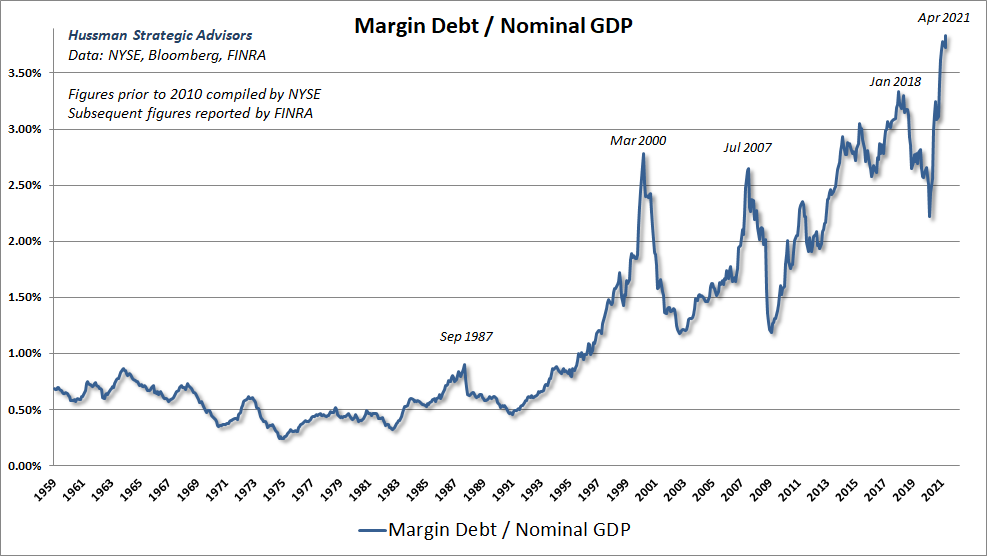
What economic activities suddenly become viable at zero interest rates that were somehow not viable before? Only projects so unproductive that any positive hurdle rate would sink them. The main activities that are encouraged by zero interest rates are activities where interest is the primary cost of doing business: leveraged real estate transactions; “carry trades” that employ enormous amounts of leverage to profit from small yield differences; and speculation on margin. Presently, margin debt as a percentage of GDP is at a historic extreme.
Again, neither loan creation, nor the issuance of securities, nor price appreciation of existing securities is sufficient to create net wealth in the economy. For that, someone needs to engage in real economic activities that draw new goods and services into existence, and have a higher value to others than the inputs that were used to produce them.
The “wealth” embodied by any security is simply the stream of cash flows that it will deliver to its holders between today and the point that the security is retired. But every security is an asset to the holder and a liability to the issuer, so securities are not “net” wealth for the nation as a whole. The true net “wealth” of a nation is the stock of productive real investments and intangible investments (education, inventions, organizational knowledge and systems) it has accumulated, plus its endowment of unused resources.
If someone’s spending exceeds their receipts, someone’s receipts will exceed their spending
Theories about money provide even more fertile ground for the emergence of incoherent ideas. These range from the idea that government deficits create “savings” (a popular idea among the MMT crowd), to the idea that there is a reliable “tradeoff” between unemployment and inflation.
Let’s begin with some very basic accounting. National output is comprised of the amount of goods and services that are consumed, plus the amount of output that is saved as “real investment” (tangible things like capital goods, factories, computers, and inventories), plus the amount consumed as government spending, plus the net amount goods and services that are exported. We can define GDP in terms of income or in terms of output, but the two definitions are essentially the same (aside from small statistical discrepancies).
From an output standpoint, investment is just output that is not consumed (even if it represents unwanted “inventory investment”). So it’s a rather obvious accounting identity that “savings” must equal “investment.” Moreover, the value of savings from an income standpoint is also equal to the value of real investment from an output standpoint.
The only thing that can make this seem complicated is that the people who “save” are typically not the same people as the ones who own the “real investment.” That’s because savings get intermediated in the financial markets. Still, in aggregate, savings always equal investment. That’s not a theory. It’s an accounting identity.
The moment the government runs a shortfall, where its consumption and net investment exceed its revenue, you know with absolute certainty that some other sector must run a surplus, where its income exceeds its consumption and net investment. Again, that’s not a theory. It’s an accounting identity.
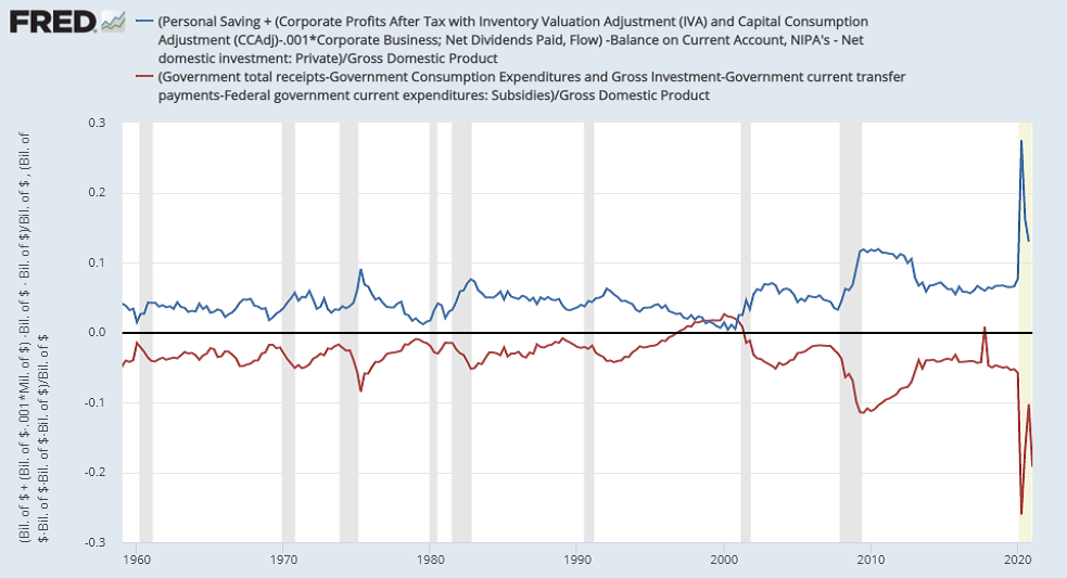
Recently, you’ve probably seen lots of headlines about “soaring” household savings, corporate profits and trade deficits, coupled with all sorts of behavioral reasons to explain it all. What may be less obvious is that these surpluses are the predictable, mechanical, mirror-images of recent government deficits.
When you see an economy where the government has run a massive shortfall over the past year, you will also see an economy where the income of other sectors, in excess of their consumption and net investment, has enjoyed a massive surplus. The chart below shows what this looks like. The negative line is just the shortfall of government revenue in funding its spending and net investment. The upper line is the aggregate surplus of households, corporations, and foreign countries. I’ve left out a few minor accounting items like net interest for simplicity, but you get the picture. The two lines are mirror images of each other. They have to be.
Moreover, we know precisely how the additional surpluses have been invested, in aggregate. Too see this, ask yourself the question – how does the government spend more than it receives in revenue? It issues Treasury securities. If the Federal Reserve buys the Treasury securities, they are replaced with base money. Who has to hold all the new Treasury securities and base money? Other sectors: households, corporations, or foreign countries. How much do they have to hold? The answer is obvious: the same amount that the government has issued to finance its shortfall.
With that, the following outcome is axiomatic: Anytime the government runs a shortfall, where its consumption and net investment exceeds its revenue, other sectors must run a precisely offsetting surplus, where their income will exceed their consumption and net investment. Moreover, that surplus must be held by those other sectors (households, corporations, and foreign countries) in the form of securities, and indeed, those additional holdings must comprise the identical securities that the government has issued in order to finance its shortfall.
Let this all sink in. There is no such thing as “cash on the sidelines” because there are no sidelines. Once “cash” is created, someone must hold it, in the form of cash, at every moment until the cash is retired. Government shortfalls don’t “create” savings. They do create “surpluses” in the sense that someone in the economy trades away some of their output in return for government securities, but this is simply a transfer of current consumption in return for securities that can be traded for consumption at another time. None of this, in itself, represents the creation of wealth. Wealth creation occurs always and only through value-added production; drawing goods and services into existence that are more valuable to others than the inputs used to produce them.
If you want an economy that creates wealth, you need an economy that directs its resources toward productive real investment and value-added production. Equilibrium gives you no other choice.
The idea that monetary and fiscal policy can be “independent” is incoherent
The government has a budget constraint. That doesn’t mean that it can’t run deficits. It just means that those deficits have to be financed. Specifically, the fiscal shortfall of government is financed by issuing government liabilities. First, new liabilities are issued by the Treasury in the form of interest-bearing Treasury securities. The Federal Reserve can then buy some of that Treasury debt and pay for it by replacing the debt with its own liabilities, which are called “base money” (currency and bank reserves). See the top of your dollar bill for details.
Unless the new base money is retired later, its creation represents a form of government finance – what economists call “seigniorage.” As Nobel economist Thomas Sargent (my other dissertation advisor at Stanford) has observed, monetary policy and fiscal policy are bound by arithmetic – “a government budget doesn’t sharply separate monetary from fiscal policy.”
On an ongoing basis, the Treasury collects existing base money from the public as tax revenue, and uses it for government expenditures. When the money is spent directly or indirectly by the government, some people give up goods and services they’ve produced, in return for payment in the form of base money collected from taxpayers.
When the government runs a deficit, it obtains funds by issuing IOUs – Treasury bonds – to the public, and then uses the base money it receives from investors to pay for expenses approved by Congress. In other words, the government obtains discretion over a portion of the goods and services produced in the economy by borrowing in the form of Treasury IOUs. Nobody would ever say that these Treasury bonds were “injected” or “pumped” into the economy. Either the government uses the borrowed funds for expenditures, or it distributes them as transfer payments or subsidies approved by Congress. In any case, whoever gets the base money gets it because Congress decided they should get it, or because they’ve given up goods and services in return for that money.
If the Fed buys the Treasury securities from someone by exchanging them with a different government liability – base money – it’s equally ridiculous to describe the transaction as “injecting” or “pumping” money into the economy. The fact is that at some point in the past, someone earned money, then lent it to the Treasury in return for an IOU, and the Federal Reserve has now simply changed the form of that liability. It’s certainly true that base money is slightly more “liquid” than Treasury securities, but it’s not “free money.”
Likewise, if the Treasury collects more base money in taxes than it uses for government expenditures, it can pay off some of its Treasury debt. If the holders of the Treasury debt are members of the public, the Treasury has just retired its IOU by shifting funds from some taxpayer to some bondholder. If the holder of the Treasury debt is the Fed, the Treasury obligation is retired, and the base money, having come home to the Fed, is also “retired.” The public has less base money, and the Fed’s balance sheet shrinks. In either case, these government liabilities are retired as the result of a budget surplus that takes in more tax revenue than expenditures.
Monetary and fiscal policy are bound by arithmetic. The total quantity of government liabilities is determined by Congress through fiscal policy. The mix of liabilities that must be held by the public – Treasury debt versus Federal Reserve base money – is determined by The Federal Reserve through monetary policy
If you read the Federal Reserve Act, you’ll find that it was written to very tightly restrict the ability of the Federal Reserve to engage in any form of money creation except by purchasing:
- liabilities of the U.S. government “fully guaranteed as to principal and interest”;
- gold and certain foreign government debt;
- commercial, agricultural, and industrial bills of exchange – essentially short-term payables secured by tangible collateral – maturing in less than 90 days, which is actually what “discounting” refers to in the Act. Notably, the Act prohibits the discounting of bills backed by “merely securities” or “other investment securities, except bonds and notes of the government of the United States;
- discounts to individuals, partnerships, and corporations, “in unusual and exigent circumstances,” as part of a program with broad-based eligibility, specifically designed “for the purpose of providing liquidity to the financial system, and not to aid a failing financial company, and that the security for emergency loans is sufficient to protect taxpayers from losses.”
Why all the rules, man? Because – and understand this clearly – if the Federal Reserve buys any security that goes belly up, and that security is not a liability of the U.S. government, the Fed will effectively have printed money to directly enrich the investors in the security that went belly up – not to provide seigniorage to the government. Purchasing any security without collateral sufficient to prevent losses would amount to engaging in fiscal policy without the authorization of Congress, and it would be illegal, not to mention unconstitutional.
That’s why the only context in which the Fed was actually authorized to buy corporate debt last year was by using a portion of CARES funds specifically approved by Congress and allocated by the Treasury. It’s why creating a shell “special purpose vehicle” to hold the debt, counting corporate debt as its own “collateral,” and valuing it at acquisition cost rather than market value, was all sharply inconsistent with the Federal Reserve Act. See for example Section 13(2) and Section 13(8), which are crystal clear that securities should not be treated as collateral, unless they are guaranteed by the U.S. government. It’s why purchasing corporate debt below investment-grade violated both 13(3) of the Federal Reserve Act and Section 4003(c)(3)(B) of the CARES Act, which imposed the requirement that collateral must be sufficient to avoid public losses. It’s also why “leveraging” CARES funds between 3x and 10x, as was first proposed, was so wildly illegal that Congress got involved to prevent it.
Mr. Chairman, if you could get back to me and just show me where the Fed has the authority to purchase these below investment-grade instruments, I’d appreciate it.
– U.S. Senator Chris Van Hollen (MD) to Fed Chair Jerome Powell, May 19, 2020
While investors believe that Fed purchases of corporate securities somehow “saved the economy,” the fact is that corporate bond purchases by the Fed last year amounted to less than $14 billion, in an economy that has over $11 trillion in corporate debt. I consider this a good outcome, given the questionable legality of the whole operation, coupled with the fact that the Fed is poorly equipped even to make collateralized business loans. The more important point is that except when the funds to do so are explicitly allocated by Congress, the Fed cannot, and should never purchase uncollateralized corporate securities, or assets of a shell entity in which uncollateralized securities are counted as “collateral.” Any loss would amount to money printing for the benefit of private investors, rather than seigniorage for the benefit of the public.
On the nature of money
Given the increased attention of investors to money, inflation, deficits, Bitcoin, market valuations, and quantitative easing, it may be useful to discuss how all of these tie together – how we can think about them in a coherent way. In the sections below, I’ve included a few charts from recent comments in order to illustrate these links.
Treasury securities and base money are both government liabilities, and they act as substitutes. It doesn’t matter that the money will never be retired. Neither, most likely, will the bonds be repaid. They’ll just be refinanced. The difference is that Treasury securities are interest-bearing, so they represent a larger liability in the long-term. It’s true that Treasury debt can be inflated away in real terms, but only if the maturity is long enough so that the interest rate can’t be adjusted higher with inflation.
Both Treasury securities and base money memorialize the fact that the government has spent more than its receipts. Someone in the economy has given up real goods and services in return for one of these liabilities, because they have confidence that they’ll be able to exchange them with someone else for future goods and services. The government can certainly destroy that confidence by engaging in too much deficit finance, and the public can certainly change the relative value they place on these liabilities. For example, if the public becomes willing to exchange fewer goods and services for a unit of base money, we call it inflation. If the public becomes willing to exchange less base money for one Treasury security, we say that nominal interest rates went up.
Why is anyone willing to hold base money at all? In my view, base money is essentially a government-produced commodity – a kind of “product” – that provides a stream of tiny transaction services to each successive holder, both as a means of payment and a store of value, provided that each holder is confident that the next person will accept it. Like any other security, the value of a unit of money can be conceptualized as the present value of the stream of all those little future transaction services. Base money has value to the public because it is involved in billions of transactions every year, its acceptance is required by fiat, embraced by convention, and it serves as the substrate for the entire banking system.
By comparison, one of the problems I have with Bitcoin is that the bandwidth of the system – about 2000 transactions every 10 minutes – is strikingly narrow, yet with extraordinarily high energy costs and coinbase dilution per transaction. There’s also the fact that a monetary system based on Bitcoin would deprive the government of hundreds of billions in seigniorage, shifting the funds that would otherwise be available for public spending to private “miners” instead. Forget that there’s neither fiat that compels others accept it, nor any reserve requirement that requires the banking system to use it. In my view the most likely cryptographic substrate of the banking system will be generated by central banks – basically just glorified base money – while independent cryptocurrencies will continue to be used primarily as a substrate for speculation and black market transactions.
It seems to me that if the perfect currency dropped from heaven and everybody agreed to use it, a big characteristic would be nobody starts off being billionaires.
– @Batbeat2
The belief that quantitative easing mechanically “supports” the market is incoherent
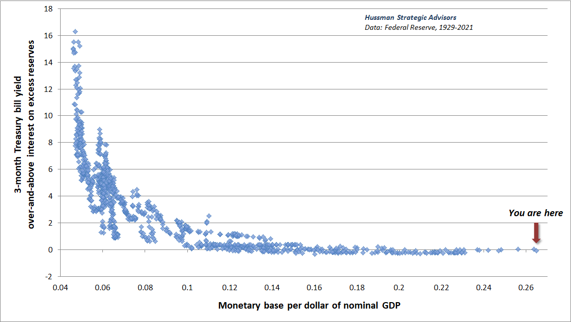
Base money and Treasury securities directly compete as forms of “short term liquidity.” If the Fed creates more zero-interest money than people want to hold, individual holders try to chase other securities that offer a pickup in yield. Of course, all of the base money still has to be held by someone, so it doesn’t go “into” those other securities. Rather, increasing the quantity of zero-interest hot potatoes causes investors to drive up the prices of closely competing securities, to the point where the “marginal” holder of money is indifferent between holding zero-interest money and low-interest Treasury debt. Here’s what his looks like. It’s my version of what economists call the “liquidity preference curve.” The more zero-interest base money investors hold relative to nominal GDP, the more inclined they are to bid up the prices of Treasury bills, driving down their yields.
Of course, the discomfort of investors who must, in aggregate, hold this mountain of zero-interest hot potatoes also encourages investors to chase riskier assets. The problem is that those assets have risk, and the moment that investors become inclined toward risk-aversion, a safe return of zero is quite preferable to a potentially severe loss. So as I’ve detailed extensively in other comments, we find that Federal Reserve easing does little or nothing to support an overvalued market once we observe deterioration and divergence (risk-aversion) in our measures of market internals, rather than broad uniformity (speculative pressure).
The chart below shows the cumulative total return of the S&P 500, partitioned by various combinations of monetary policy and market internals (our main gauge of speculative vs. risk-averse psychology).
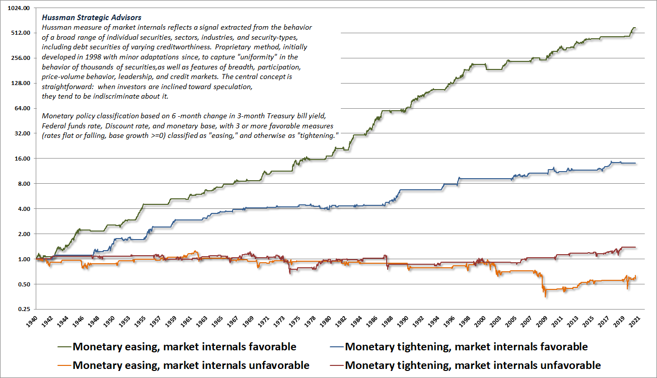
Put simply, it’s not quantitative easing that holds the market up. It’s the belief that quantitative easing holds the market up that holds the market up. The problem is that the whole operation relies on the absence of risk-aversion among investors. In my view, it’s best to attend to the uniformity or divergence of market internals directly.
The belief that monetary policy determines inflation is strikingly incomplete
There are two key reasons you’ll find a very weak relationship between the money supply and the rate of inflation (and you will). The first is that monetary policy doesn’t actually determine the quantity of government liabilities that the public must hold, nor does it determine the confidence of the public in those liabilities. Fiscal policy does that. Monetary policy simply changes the mix of government liabilities – how much the public must hold as Treasury bonds, and how much the public must hold as base money.
The key is that both liabilities share the same basis for public confidence – the implicit expectation that the issuance of government liabilities won’t exceed the growth of the real economy so profoundly and consistently that others will become unwilling to accept these pieces of paper in return for a (reasonably) stable quantity of goods and services.
The second and related reason you’ll find a weak relationship between the money supply and the rate of inflation is that inflation has an enormous psychological component. The public appears to be quite tolerant of short-term fluctuations in the relative supply of government liabilities (bonds and base money) versus goods and services, but if new issuance of government liabilities becomes large enough to trigger psychological “revulsion” toward that new supply – particularly if the economy faces constraints in producing new goods and services – inflation typically follows.
If inflation is running out of control, monetary policy doesn’t stop it simply by reducing the growth rate of money. It’s certainly true that rising interest rates can aggravate recessions and disrupt financial markets, so tight money can be enough to disrupt ordinary cyclical inflation pressure. But if you examine periods of aggressive and sustained inflation both in the U.S. and across countries, you’ll find that tight monetary policy stops inflation mainly by imposing a tighter and more credible constraint on fiscal policy – by removing the printing press as a form of government finance, and thereby increasing the confidence of the public in government liabilities generally.
In each case that we have studied, once it became widely understood that the government would not rely on the central bank for its finances, the inflation terminated and the exchanges stabilized. We have further seen that it was not simply the increasing quantity of central bank notes that caused the hyperinflation. Rather, it was the growth of fiat currency which was unbacked, or backed only by government bills, which there never was a prospect to retire through taxation.
– Nobel economist Thomas J. Sargent
From an economic standpoint, we can think of the general price level in terms of two “marginal utilities” (the extra happiness you get from having one extra unit of something). If you get 10 units of happiness from an ice cream cone, but only 2 units from a pencil, then the price of one ice cream cone (pencils/cone) should be five pencils. In theory, the price level is the “marginal utility” of one unit of goods and services divided by the marginal utility of one unit of money.
Price level = Marginal utility of goods and services / Marginal utility of money
So what drives inflation? Well, the “marginal utility” of goods increases either when the desirability of goods and services increases, or when the supply of goods and services is constrained. The “marginal utility” of money and government liabilities falls either when their desirability to the public falls, or when their supply is expanded. Half of those considerations depend on relative supply, and half are wholly psychological. Historically, and across countries, the best recipe for inflation has been expansion in government deficits coupled with either output constraints or a supply shock.
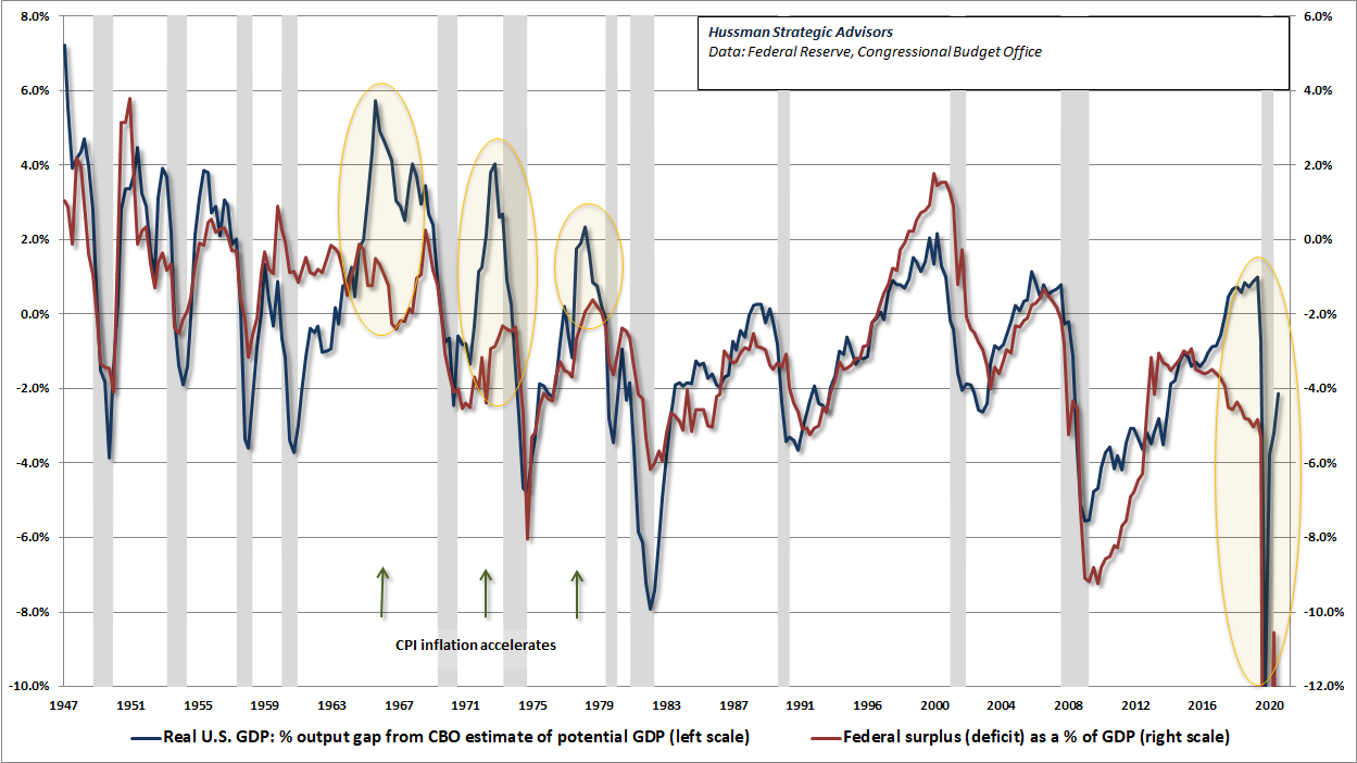
The chart below shows the GDP output gap (real GDP relative to “potential” GDP as estimated by the CBO) alongside the U.S. government deficit as a share of GDP. It’s clear that deficits fluctuate with the economic cycle, and this alone doesn’t disrupt confidence in government liabilities. In contrast, we tend to see inflationary pressure when deficits become what I call “cyclically excessive” relative to the output gap, and output is running close to potential (or supply constraints become problematic as they have in recent months).
What drives deflation then? Push marginal utilities in the other direction. The marginal utility of goods and services can decline if people become less inclined toward current consumption, or if goods and services are in ample supply. In a rapidly growing economy, you’ll find that stronger output growth is actually associated with lower inflation, because the expanding supply of goods places downward pressure on the marginal utility of goods. In a credit crisis, safe liquidity can become a desirable asset – its marginal value increases, and you get deflationary pressures. Constraining the supply of government liabilities can also raise their marginal utility.
You can’t reliably model these things in some linear way. Just like stock prices, part of the value is based on “fundamentals,” and part is based on psychology. Your best bet is to monitor both, and to pay particular attention when financial assets associated with inflation expectations begin to perk up uniformly. It’s an unfortunate reality, but the best predictor of future inflation is actually current inflation.
Presently, we’ve got enormous government deficits, coupled with economic and labor market frictions as the economy gradually reopens. That alone has created clear short-term inflation pressures. The question is the extent to which deficits will continue, for what purposes, or how durably various supply frictions will persist. All of these matter for the future course of inflation. It will be important to monitor inflation-sensitive market gauges for signs of revulsion and deteriorating confidence.
I would be particularly concerned about deficits that are not clearly related to expansion in productive capacity (such as infrastructure, research & development, or clean energy). Productive forms of deficit spending, like any sort of productive spending, can certainly justify the use of debt, because the debt can be repaid from future value-added production. Still, the size of recent deficits is of clear concern, as is the Federal Reserve’s encouragement of deficits by monetizing them.
Even if large deficits don’t result in current inflation, it’s important to notice that once government liabilities are created, they stick around until they’re retired. It’s quite possible that we could create an enormous volume of government liabilities in a weak economy without immediate inflation, yet discover later that the overhang of these liabilities (both Treasury debt and base money) could contribute to high inflation later, because their quantity has become disproportionate to the volume of real goods and services produced by the economy.
The popular interpretation of the Phillips Curve is a misconception
As a former academic economist, I’ve often noted that academic economists don’t actually study the economy. They study “economies” – as in – “Consider an economy where there are two islands, a turnpike, and five guys named Bob, one who is the government but nobody knows which one.” As a graduate student at Stanford, I once attended a seminar where a young Paul Krugman described a model as he casually drew a few arrows on the blackboard. A faculty member demanded that he either explicitly describe the dynamics or erase the arrows. The interchange escalated with breathtaking speed, ending with the faculty member pounding the desk, screaming “ERASE THE ARROWS!” and then storming out, slamming the door behind him.
Amid the multiple personality disorder of policy-makers that oscillates between simplistic but weak-fitting “Phillips Curve” dogma and wildly elaborate but weak-fitting “dynamic stochastic general equilibrium” models, the durable constant is that policy-makers don’t focus much of their thinking on the actual economy either. Instead, they think in terms of theoretical “objects” that take on lives of their own, and offer “policy levers” based on hypothetical relationships rather than data. This avoids any need for evidence that the policies actually have reliable and sizeable effects, much less historical context.
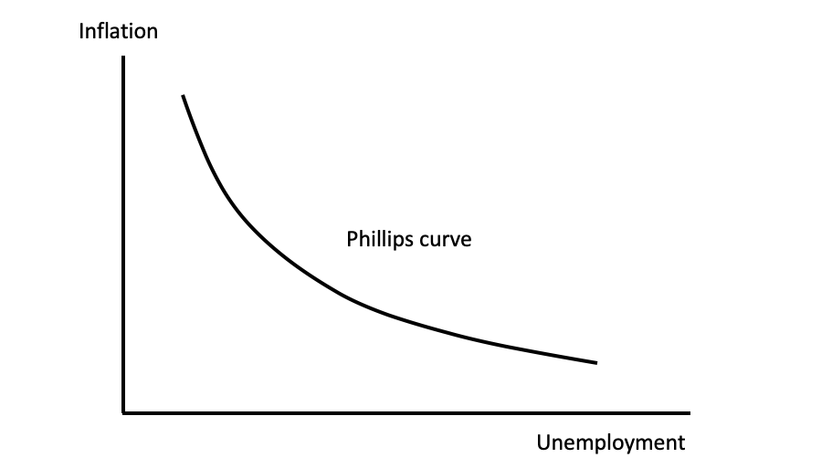
Think that’s an exaggeration?
Here’s the Phillips Curve you might have seen in your college textbook, and the same one that’s in the heads of policy makers at the Federal Reserve. It’s very pretty, and it immediately seduces the observer to imagine the ample social benefits that could be engineered if we could just “achieve” a higher rate of inflation.
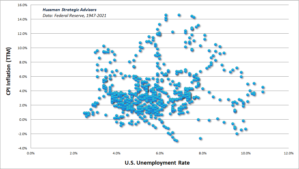
Unfortunately, the data are not so kind. Here’s the actual scatterplot. First, unemployment versus trailing 12-month inflation.
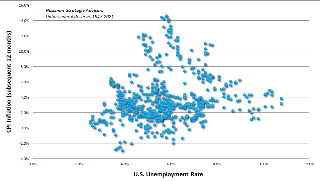
Next, unemployment versus subsequent 12-month inflation.
Finally, for good measure for those who imagine that lower unemployment can be “bought” with higher inflation, here is a scatter of trailing 12-month inflation versus the unemployment rate one year later.
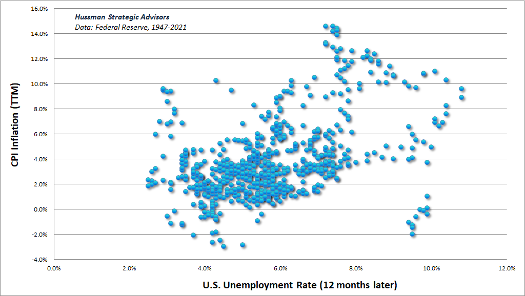
Try as one might to salvage this theory with “expectations augmented” features, leads, lags, advanced econometrics, and theoretical modifications, you’ll have a difficult time finding any useful relationship at all between the rate of unemployment and the rate of general price inflation (e.g. the consumer price index). You can torture the data enough to give you a significant p-value or F-test, but it’s much harder to demonstrate that extraordinary monetary policy has an effect size that’s worth the financial distortions. It’s just impossible to salvage much when an economic relationship that policy makers treat as a tidy curve is actually a disorganized shotgun scatter that slopes in the wrong direction.
Part of the problem is, or should be, immediately apparent to anyone who has just enough intellectual curiosity required to simply read the title – just the title! – of A.W. Phillips’ famous 1958 paper: The Relation Between Unemployment and the Rate of Change of Money Wage Rates in the United Kingdom, 1861–1957.
See, here’s the thing. The Phillips Curve was actually a statement about wage inflation, not general price inflation. Moreover, Phillips studied a period when the U.K. was generally on the gold standard, so general price inflation was very stable. In fact, Phillips makes an explicit point of “ignoring years in which import prices rise rapidly enough to initiate a wage-price spiral.” So the wage inflation Phillips was observing was actually real wage inflation; inflation in wages relative to the prices of other things.
Put simply, the Phillips Curve that policy makers imagine in their heads is incoherent. It doesn’t actually exist. The actual relationship that Phillips found was a rather straightforward relationship between the scarcity of labor and the price of labor (relative to other things). When unemployment is high and labor is plentiful, real wage inflation tends to be muted. When unemployment is low and labor is scarce (particularly in situations like today where there are labor market frictions as the economy recovers from the pandemic), real wage inflation tends to accelerate.
The mapping between observable valuations and expected returns is independent of the level interest rates
Suppose I hand you an IOU that will deliver, with certainty, $100 a decade from today. The current price is $32. Given this information, it’s simple to calculate that your expected annual return is:
($100/$32)^(1/10)-1 = 12%.
Did you need to check the level of interest rates to do that calculation? No, you did not. You can certainly compare that expected return with the prevailing level of interest rates, but that’s optional.
Now suppose I tell you that the price of the IOU is $82. Again, it’s simple to calculate that your expected annual return is:
($100/$82)^(1/10)-1 = 2%.
It’s essential to understand this point: the mapping from observable valuations to expected returns does not need to be “adjusted” for the level of interest rates. You’re free to compare the expected return with interest rates if you like, but once you have an estimate (or sufficient statistic) of future cash flows and the current price, nothing else is required to estimate the expected return.
The reason so many investors and even professionals are confused on this point is that they have conflated it with an entirely different problem. Suppose that we know the expected cash flows but the current price is unobservable or excluded from our calculations. What’s the “fair” price we should pay for the security? Well, it depends on the rate of return we want to earn. At this point, you might look around and say, well interest rates are so-and-so, and I’d like to get a few percent more than that, so maybe I’d be ok with a 4% return. Fine. Now we can plug that in, and we get a target price of:
$100/(1.04)^10 = $67.56.
So here’s the rule. If you’ve got a reliable valuation measure that relates the current price to some fundamental that’s reasonably representative of future cash flows, the expected return can be estimated directly. Comparing that expected return to interest rates comes later, and is optional.
In contrast, if you’ve got an estimate of future cash flows and you don’t know the price, you can use the level of interest rates, if you wish, to help you decide what a “fair” return might be, and the price that would produce that expected return.
Don’t confuse those two problems.
When analysts say that extreme valuations are “justified relative to interest rates,” they are actually saying that dismal expected returns on stocks are “justified” by dismal returns on bonds. Nothing more. If it makes you feel better, you can certainly repeat the phrase in the mirror as your morning affirmation, but it won’t make your future passive returns on stocks any less dismal.
Put simply, extreme valuations imply poor expected returns, and those returns aren’t mitigated by low interest rates. Rather, the combination of poor expected returns on both stocks and bonds leaves passive investors absolutely worse off, because it deprives them of alternatives.
I know many of you don’t believe that, so let’s look at the data in three dimensions. The chart shows valuations on log scale, along with the level of long-term Treasury bond yields, and the actual subsequent 12-year total return of the S&P 500. The current point can’t be plotted, because we don’t know actual subsequent 12-year total return yet, but the two observable variables – valuations and interest rates – would put us in the extreme lower corner of this plot.
Now, looking at the chart, it might seem that low interest rates are reliably associated with extreme valuations, but that’s actually not true at all. Rather, valuations drive the expected returns so strongly that the interest rate information adds virtually no information at all. The points just lie behind the principal scatter at varying distances. To see this, I’ve also provided a view of the same scatter from the top-down.
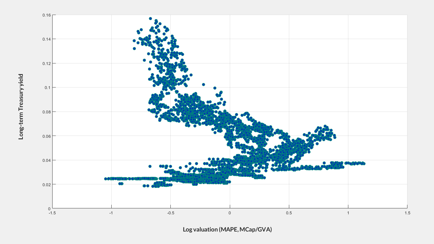
Notice something. When interest rates have been extremely high (above 10% or so), valuations have been reliably low. But at rates below 10%, there is no reliable relationship between interest rates and valuations.
Here’s a fascinating result (h/t Jeff Huber for proposing the question): When we examine the relationship between valuations alone and subsequent returns, we find a correlation of 0.9170 in data since 1928. If we add the level of interest rates as an additional explanatory variable, we get no improvement in that correlation. What surprised even me is that if we add a third variable – the change in interest rates over the coming 12-years (which assumes that we know future interest rates with certainty) – the correlation rises to only 0.9174.
Put simply, once you know the level of valuations, at least for reliable valuation measures, knowing the current level of interest rates – and even knowing the future level of interest rates – does not improve your projection of future returns. Once you’ve estimated the future cash flows, and you know the current price, you can estimate expected long-term returns directly. The level of interest rates is irrelevant to that arithmetic. You can compare your estimate of long-term returns with the level interest rates afterwards, if you like, but interest rates are not required for the calculation. That’s clearly true in theory, as I noted at the beginning of this section, but I was still surprised by the degree that it was true in the historical data, even at a 12-year horizon.
One can certainly imagine factors that might weaken this result, particularly at short horizons, but even then, nearly 100 years of historical data suggest that attending to the combination of valuations and market internals is an adequate basis to navigate market cycles over time. As I’ve noted before, the only thing that was truly “different” about recent years is that we had to abandon our response to historical “limits” to speculation. Instead, we’ve become content to gauge the presence or absence of speculation or risk-aversion, without assuming any well-defined limit to either.
There’s one way to formulate the valuation problem that does require one to consider the level of interest rates. That consideration comes in when you’re trying to estimate the likely difference in expected returns between stocks and bonds. As I’ve noted before, I am not a fan of “equity risk premium” models that divide the earnings yield of stocks by the interest rate or subtract the level of interest rates from some measure of stock yields. Both of those operations assume a very structural, one-to-one relationship between the valuation of stocks (which are very long-duration instruments) and the valuation of bonds (which have a far shorter durations except when equity valuations are profoundly depressed).
Instead, our own equity risk premium estimate is straightforward: use valuations to estimate expected equity returns for a given investment horizon, and then compare that estimate with the yield-to-maturity of bonds for that same investment horizon. I’ve seen no alternative method of estimating the equity risk premium (including Shiller’s “excess CAPE yield”) that is better correlated with the actual difference between stock and bond returns across history. Still, as we observed for the 12-year period following 1988, actual returns can be far better than one would have projected if the end of the period happens to be the peak of a bubble. The dismal forward-looking returns here are the mirror image of glorious backward looking returns. The same outcome followed the 1929 and 2000 valuation extremes.
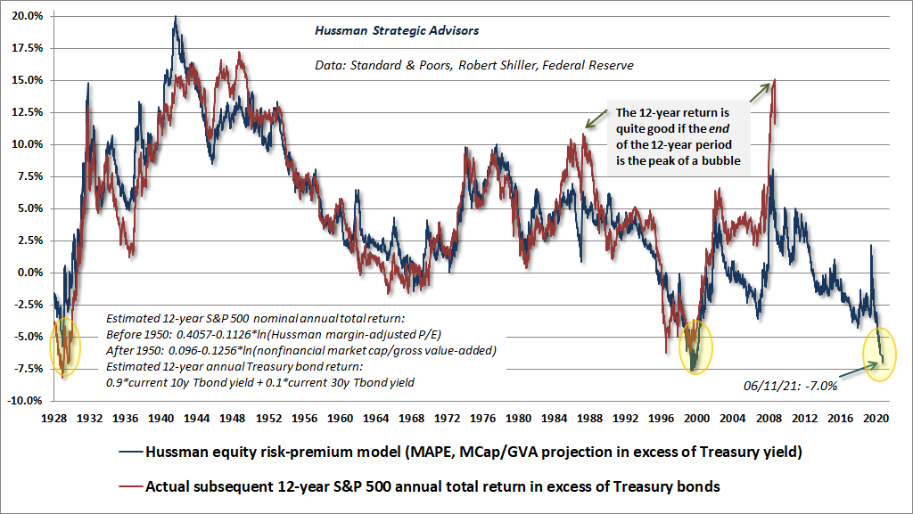
By the way, take a moment to notice how widely the difference in returns between stocks and bonds has varied across history. If low interest rates were always associated with steep valuations, and high interest rates were always associated with depressed valuations, you would not observe much variation in this chart. The fact that the expected and actual “premium” fluctuates all over the place means that there are distinct periods where either stocks, or sometimes bonds, are vastly preferable to the other. In some cases, cash can also provide “option value,” at least until a retreat in valuations or an improvement in market action provides an opportunity to embrace greater market risk. Rather than cash positions, I prefer hedged equity in these situations. Two years ago, I published a white paper titled Strategic Allocation, describing how we can use this information in a disciplined way.
Competitive free enterprise without the erosion of excess profits is not competitive free enterprise
If we examine the history of economic growth, it is clear that the long-term expansion in the standard of living does not simply reflect the continuous increase in the production of some single “representative good,” but instead by the progressive introduction of new inventions, technologies, and products that satisfy previous unmet needs. In his work on economic development, Joseph Schumpeter recognized the critical role of entrepreneurs in advancing this process.
When Schumpeter described “creative destruction,” and Adam Smith described the “invisible hand,” they envisioned an economic system where the potential for profit would serve as an incentive for innovation by those who were best capable of filling unmet needs. But they also saw profits as inherently self-destructive, because profit opportunities would encourage a “swarm-like” activity of other entrepreneurs. That competition would expand production, and simultaneously produce economic growth while eroding excessive profits.
As the rise and decay of industrial fortunes is the essential fact about the social structure of capitalist society, both the emergence of what is, in any single instance, an essentially temporary gain, and the elimination of it through the working of the competitive mechanism, obviously are more than ‘frictional’ phenomena, as is the process of underselling by which industrial progress comes about in a capitalist society and by which its achievements result in higher incomes all around.
– Joseph Schumpeter, The Instability of Capitalism (1928)
It is not from the benevolence of the butcher, the brewer, or the baker that we expect our dinner, but from their regard to their own self-interest. He generally neither intends to promote the public interest, nor knows how much he is promoting it. He intends only his own gain, and he is, in this, as in many other cases, led by an invisible hand to promote an end which was no part of his intention.
– Adam Smith, The Wealth of Nations
One of the concerning aspects of current economic debates is the tendency to embrace “capitalism” indiscriminately, without actually considering the aspects of this system that contribute to growth and widespread prosperity. To parrot Churchill’s statement that “capitalism is the worst economic system, aside from all the others” is incoherent. Well, partly because he never said it. What he did say was “Democracy is the worst form of government except for all those other forms that have been tried,” and he attributed it to someone else. But the statement about capitalism is also incoherent if one becomes willing to dispense with the very features of capitalism that drive growth and lift all boats.
Personally, I prefer the phrase “competitive free enterprise” to “capitalism” because it clarifies things – particularly the essential role of entrepreneurship, and also the role that free entry and competition should have, but not always does, in eliminating excessive profits over time. A careful understanding of free enterprise must also consider “externalities” where the behavior of an individual or company imposes costs to others that they do not bear (e.g. pollution), or provides benefits to others that they do not fully capture (e.g. education, scientific research). There’s little question, for example, that Amazon is extraordinarily efficient in meeting customer needs, but there is also little question that by channeling resources out of the local circular flow, the resilience of countless communities is subtly weakened. The costs are not borne by Amazon, nor is the damage per transaction high enough for any customer to change their behavior.
Likewise, international trade can have features that amplify systemic inequity or impose uncompensated harm to others. All of these are “externalities.” In these cases, a free market will produce too much of the activities that produce negative externalities, and insufficient amounts that produce positive externalities, unless policies are introduced to impose private costs for harmful activities or subsidize beneficial ones (e.g. carbon taxes, investment tax credits, applying sales or value-added taxes to out-of-community purchases and reinvesting them back into the community). Nobel economist Ronald Coase demonstrated policies that “internalize” these externalities can enable competitive free enterprise to produce more efficient outcomes with no loss of overall welfare.
A well-known difficulty emerges in the case of monopoly. In the traditional analysis of monopoly, excess profits are preserved by the ability of the monopolist to restrain output and thereby maintain prices at higher levels than would exist in a competitive economy. In the standard analysis, increasing levels of output are associated with a rising marginal cost for each additional unit, so the monopolist has an incentive to hold output at a sufficiently limited level to ensure a wide gap between marginal revenue and marginal cost. So monopolists are traditionally thought of as producers that charge high prices and limit supply.
However, in any setting where the marginal cost of producing each additional unit declines with the level of output, simply obtaining more customers is sufficient to enhance profits. In this case, neither limited supply nor high prices are required, yet the company may enjoy the status of a “natural monopoly.”
The level of profits in this case may have little relationship to the contribution of the entrepreneur, but may instead reflect broader factors such as network effects, social dynamics, and general technological efficiencies that were no part of the entrepreneur’s invention. Undoubtedly, the introduction of a new and useful product is deserving of compensation, possibly even extraordinary reward. Without it, the entrepreneurial incentive would be weakened. Yet when the act of invention is amplified by such powerful network effects that enormous natural monopolies result, much of the profit and enterprise value of these monopolies represent private claims to very general features of technology, network effects, social conventions – sometimes even physics and genetics – that might be better characterized as public goods.
Suppose a new technology like quantum computing emerges, and it’s now possible to create intelligent robot toasters that can do every possible thing that human labor can accomplish, from manufacturing, to teaching, to art; better and more cheaply than any human counterpart. Even better, robot toasters can reproduce at nearly zero “marginal cost,” and become more effective every time the toasters interact with each other. Suppose that even though many people could create them, I happen to be first, and no other entrant can successfully compete once my toasters start interacting. In that world, I and my army of robot toasters may be able to “efficiently” produce all of the output in the economy, and gradually accumulate all of its resources. Others may be able to survive by going into debt or indenture. None of this monopolistic behavior could be considered to be competitive free enterprise.
Weakening “creative destruction”
In Schumpeter’s framework, the emergence of significant innovations provokes the “swarm-like” entry of new entrepreneurs that operate alongside older enterprises. The resulting boom results disrupts the previous equilibrium and inevitably results in errors, speculation, and debt issuance by new and older businesses alike, which can later contribute to subsequent recessions – “Part of the debt structure will crumble. Freezing of credits, shrinkage of deposits, and all the rest follow in due course.”
As new competitors emerge to take advantage of what Schumpeter viewed as extraordinary but “essentially temporary” profits, output and employment expand, profits fall back to normal levels. This continual cycle of “creative destruction” drives productivity growth, employment, and income across the economy, though not without periodic disruptions and crises.
The economic cycles of recent decades have included many of these features, but the process has also been regularly short-circuited by monetary policies that treat all borrowing as productive borrowing, and all business failure as unacceptable failure. The combination has since contributed to an overly indebted corporate sector, a global financial crisis, and an extended period of labor market slack where wages were depressed and profits became entrenched, without their elimination “through the working of the competitive mechanism.” Meanwhile, nearly every aspect of Federal Reserve policy has contributed to an enormously skewed wealth distribution, where corporate securities are valued at extreme multiples of their underlying cash flows.
One of the problems with the current economic equilibrium is that some industries no longer reflect “competitive free enterprise” and appear much closer to “natural monopoly.” When people hear the word “monopoly,” they typically think of the cartoon guy with a top hat on the Hasbro game, where the object of the game is to corner the market and soak the other players. But a “natural monopoly” can occur in any business where the “marginal cost” – the cost of producing one extra unit – declines as output increases. In that situation, adding another customer always increases your profits provided the new customers aren’t costly to acquire. You don’t have to soak them. You just have to acquire them.
The key to riches in this game is to find some way to distribute your efforts over the largest possible number of individual “units.” Show me a multi-billionaire, and I’ll show you someone who is benefiting not just from their own “invention” but from distribution systems, network effects, and features that resemble natural monopoly. There’s nothing inherently nefarious about that. It’s just that there’s a point where treating it all as individual “wealth” and personal achievement strains reason, particularly when the tax system treats profits, carried interest, and financial gains as sacrosanct. A tax system that treats multi-billion dollar equity holdings as absolutely untouchable because they’re “unrealized” is a political choice, not an economic one.
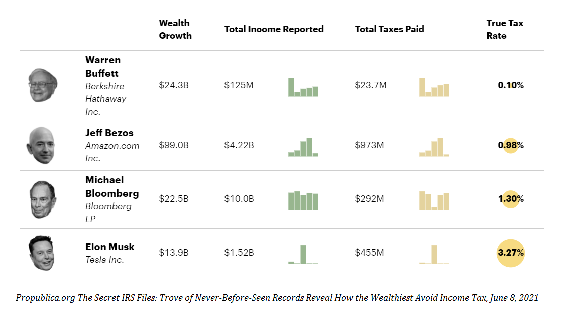
Natural monopoly is how we’ve found ourselves in a world where a handful of individual companies account for a quarter of U.S. market capitalization. One might imagine that this is an investment opportunity if not for the fact that all of these companies are trading at wildly elevated multiples of those already inflated fundamentals. The chart below shows the median price revenue ratio of the largest and smallest 10% of S&P 500 components by market capitalization. Compared with recent extremes, the pre-crash bubble peak in 2000 was a picnic.
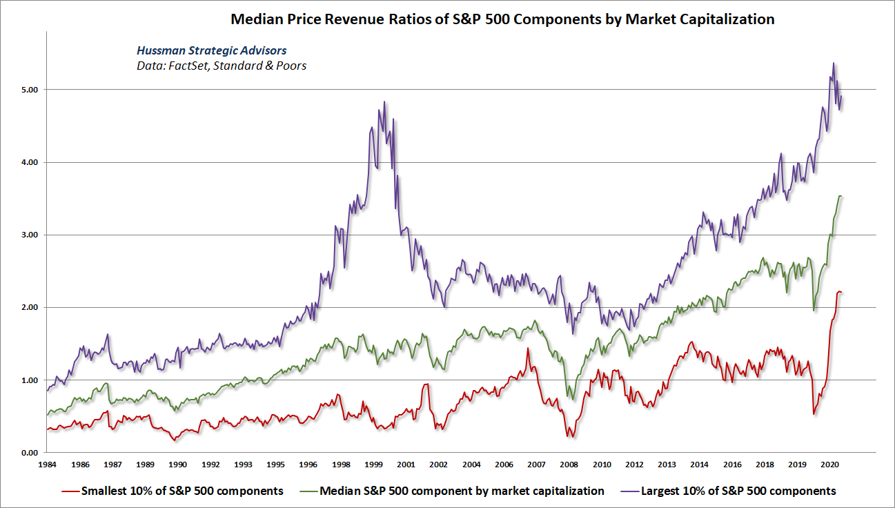
Still, even as part of the economy is behaving as a wildly overvalued natural monopoly, non-financial profit margins are starting to normalize to a greater degree than investors may recognize (particularly when one excludes massive but temporary pandemic relief subsidies). Across the non-financial sector as a whole, real unit labor costs have begun to rebound in the past few years, which has started to pressure profit margins lower. Unfortunately, this is occurring at a point where weaker profit margins threaten to cause credit strains for the mountain of debt that was taken on in the interim.
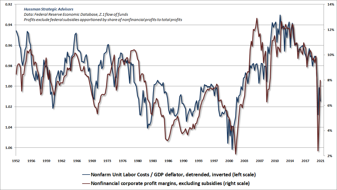
One of the polarizing political debates here is the extent to which extraordinary profits should be taxed. Schumpeter argued that invention and entrepreneurial activity can be conceived as a means of production, and as such, that part of the value of new products should be imputed to it. In that sense, profits don’t necessarily reflect any “exploitation” of labor, but are instead compensation deserved by an important factor of production. Still, Schumpeter didn’t distinguish between the portion of the entrepreneurial activity that involves actual invention, and the portion that reflects network effects, economies of scale, amplifiers, feedback loops, social convention, and similar factors that – in practice – account for the lion’s share of profits for natural monopolies like Facebook, Amazon, Google, and numerous other companies.
Undoubtedly, the act of invention deserves compensation, and this compensation can be significant when an invention has achieved near-monolithic success. But at some point – my personal impression circulates around a few billion dollars at best – the value attributable to the hard work and effort of the inventor stops, and the remainder captures network effects and scale economies that might be more accurately considered “public goods” than private innovations.
For example, Facebook is successful largely because a computer program written by a small initial team began drawing in users (original product: a “Hot-or-Not” clone called FaceMash to rate pictures of Harvard students without their permission). Those early Facebook users drew in friends, who use it because other people they know use it, and the platform gradually became the “black hole” of social networks, pulling everyone in toward it. There’s undoubtedly value that can be imputed to the platform itself, but a great deal of the value is attributable to network effects.
Capital with a “K” is not capital with a “c”
Another subtle feature of the current economic landscape is the subtle but very intentional blurring of the word “capital.” In economic theory, output is often described as being a function of labor L and capital K, where “capital with a K” means real, productive investment like equipment, factories, and can even be extended to inventions. Because accumulating productive capital K also increases the productivity of labor L, and the amount of output that labor can command, there’s a good deal of economic literature that encourages low taxes if any, on capital K. Of course, in the United States, real productive investment can be depreciated and deducted over time, so it isn’t taxed at all.
The subtle blurring comes in when people talk about financial capital “capital with a c” as if it is the same thing as K. Financial capital with a c involves things like debt, equities, interest, and profits. Certainly, all of these are involved in financing capital with a K, but again, K isn’t taxed at all. Beyond that, there’s absolutely no reason that a dollar of income earned from trading stocks and bonds should be taxed any differently than a dollar of income earned as wages or salary. When people yammer on with phrases like “We shouldn’t penalize capital formation,” they’re really taking an argument about productive capital K, and blurring it as if it also applies to purely financial capital c.
Look, I’m all in favor of tax incentives and accelerated depreciation for productive “capital with a K” – equipment, factories, research & development, clean infrastructure, and even forms of human capital like education – but the idea that profits, carried interest, and financial gains are somehow fundamentally different and more preferable than wage income is a disingenuous bifurcation of the word “capital.”
That’s yet another reason I prefer the phrase “competitive free enterprise” to “capitalism.” When people say the word “capitalism,” half the time they don’t even know which kind of capital they’re talking about. In a properly functioning competitive free-enterprise system, profits are incentives for innovation, market entry, and growth. But they are also – and should be – the engines of their own creative destruction. When economic policies treat profits as sacrosanct, and treat financial gains as somehow preferential to wage income, it’s no wonder that the end result is low real structural growth coupled with breathtaking income disparities.
An imbalance between rich and poor is the oldest and most fatal ailment of all republics.
– Plutarch, 100 A.D.
I’ll say this again. When you net out all the assets and liabilities in the economy, the only thing that remains is our stock of productive investments, inventions, education, organizational structures, and unconsumed natural resources. Those are the basis of our national wealth. Every security is both an asset and a liability, and in aggregate, they net to zero. Moreover, since every security must be held by someone until it is retired, the value of that security is ultimately determined by the long-term stream of cash flows that it delivers to the holder. Overvaluation doesn’t create wealth. It simply enables a wealth transfer from others, and only then if a holder actually sells at the elevated price. We would be much stronger as a nation if were capable of focusing on what’s real, what’s productive, what’s equitable, and what has the capacity to lift all boats. That can be one of the virtues of competitive free enterprise, but it’s also something that we are quite capable of destroying if we forget how it all actually works.
My 5/18/21 Op-Ed in the Financial Times:
The myths behind the current stock market bubble
A quick accounting note on “shortfall” versus “deficit”: Consider two sectors, government (g) and private (p).
The equation below says that the shortfall of government is equal to the “surplus” of the other sectors:
Consumption_g + Investment_g – Revenue_g = Revenue_p – Consumption_p – Investment_p
Rearranging, the equation below says that the total investment is equal to total saving:
Investment_g + Investment_p = (Revenue_p – Consumption_p) + (Revenue_g – Consumption_g)
As for how various items fit together, gross government spending equals government consumption and net investment, plus government transfer payments to individuals, plus subsidies (transfers to goods and services producing enterprises), plus interest payments. In describing the relationships of sectoral surpluses and shortfalls, I use the word “shortfall” instead of “deficit” because I’ve moved certain government expenditures such as transfer payments, subsidies, and interest into private income. In this way, the words “surplus” and “shortfall” consistently describe the income of a given sector relative to its own consumption and net investment.
Keep Me Informed
Please enter your email address to be notified of new content, including market commentary and special updates.
Thank you for your interest in the Hussman Funds.
100% Spam-free. No list sharing. No solicitations. Opt-out anytime with one click.
By submitting this form, you consent to receive news and commentary, at no cost, from Hussman Strategic Advisors, News & Commentary, Cincinnati OH, 45246. https://www.hussmanfunds.com. You can revoke your consent to receive emails at any time by clicking the unsubscribe link at the bottom of every email. Emails are serviced by Constant Contact.
The foregoing comments represent the general investment analysis and economic views of the Advisor, and are provided solely for the purpose of information, instruction and discourse.
Prospectuses for the Hussman Strategic Growth Fund, the Hussman Strategic Total Return Fund, the Hussman Strategic International Fund, and the Hussman Strategic Allocation Fund, as well as Fund reports and other information, are available by clicking “The Funds” menu button from any page of this website.
Estimates of prospective return and risk for equities, bonds, and other financial markets are forward-looking statements based the analysis and reasonable beliefs of Hussman Strategic Advisors. They are not a guarantee of future performance, and are not indicative of the prospective returns of any of the Hussman Funds. Actual returns may differ substantially from the estimates provided. Estimates of prospective long-term returns for the S&P 500 reflect our standard valuation methodology, focusing on the relationship between current market prices and earnings, dividends and other fundamentals, adjusted for variability over the economic cycle.