Equilibrium and the Dentist in Poughkeepsie

 

John P. Hussman, Ph.D.
President, Hussman Investment Trust

March 2026

---

When we try to pick out anything by itself, we find it hitched to everything else in the universe.

– John Muir, Scottish-born American naturalist and writer

When we think of the word “equilibrium,” a whole range of meanings may come to mind

“Supply equals demand.” (market clearing)
“All deficits and surpluses add to zero.” (accounting identity)
“Things are temporarily stable, with no impetus to change.” (steady state)
“Every action has an equal and opposite reaction” (Newton’s Third Law)
“Nature keeps perfect books. What changes on one side is balanced on the other. Every change in spin, charge, and momentum in one place is exactly accounted for elsewhere, so the totals never change.” (Law of conservation)
“Nothing is lost, nothing is created, everything is transformed. (Lavoisier’s maxim)

The word “equilibrium” is an invitation to recognize that nothing exists by itself, alone. Subject and object are two sides of the same coin – their interaction is a single phenomenon.

Even at the tiniest level of the universe, if we look at the polarization of two entangled photons, the spin of two electrons, or the state of two qubits in a quantum computer, we find that measuring one immediately determines the correlated outcome for the other, even far away, without sending any signal. While there’s no theoretical limit to entanglement, the record distance measured to date was between two entangled photons – separated by 747 miles – which is kinda cool.

All of this may seem very abstract, but we can see that the workings of “equilibrium” pervade even the most ordinary aspects of daily life.

At the most basic level, for example, we realize that there’s no such thing as a buyer putting cash “into” the market without a seller taking that same cash “out of” the market. Every share someone just bought is a share someone else just sold (or issued). The buyer, the seller, and the exchange are inseparable – their interaction is a single phenomenon. Talking about “cash going into the market” is like talking about the sound of one hand clapping.

This month, we’ll examine a whole range of examples involving equilibrium, all of which are directly relevant to current economic and market conditions. First, we’ll review the strikingly lopsided equilibrium that’s emerged across various sectors of the economy. This equilibrium helps to understand the record level of corporate profits in recent years – although the distribution of corporate profits is more closely related to whatever innovations and industries are dominant at any particular point in time.

Next, we’ll examine equilibrium in the securities markets – why prices fluctuate, what “flows” actually mean, and how fundamentals, information, and investor beliefs collaborate to determine prices and trading volume.

We’ll then examine the current insensitivity of investors to valuations, and what aspects of the current speculative bubble can and cannot be well-explained by passive “money flows.”

Finally, we’ll share some perspectives, rooted in finance theory, that help to understand how “glamour” companies gain market capitalization, and the beliefs behind the “bubble on a bubble” that we’ve seen in the information technology in recent years.

We’ll do more than the usual amount of math, because equations impose discipline – allowing us to escape from the muddy trap of hidden assumptions and verbal arguments that can often sound very convincing. If you’re already reaching for an Epi-Pen, don’t worry, just read around the math, and know it’s there to support systematic analysis, so we don’t get caught in the mud.

Corporate profits and household deficits

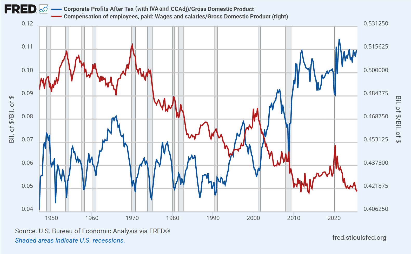
One of the defining features of the present state of the U.S. economy is the striking gap between the prosperity of corporations and profitability on one hand, and the increasingly tenuous financial condition of working families that rely on wage and salary income.

The discussion below expands on the January comment, which focused on the equilibrium that relates record corporate profits – directly, and as an accounting identity – to mirror image deficits in the household and government sectors (see How the Bubble Manipulates Time). Once we understand the causes and conditions that allowed recent record profits to “manifest,” we are also better prepared, and will be less surprised, when things change.

Thinking in terms of equilibrium helps to understand exactly why and how corporate profits have increased to a record share of GDP in recent decades. The reason isn’t growth-enhancing productivity. Since 2000, real U.S. GDP growth has expanded at the slowest 25-year growth rate in U.S. history, despite profound technological change. The main impact of technology has not been to increase economic growth, but to widen the wealth distribution. What’s really going on is so striking that once you see it, you can’t “un-see” it – the deficits of one sector always emerge as the surplus of another.

The chart below shows corporate profits in excess of net investment in blue, with the mirror image deficit of other sectors – primarily households and the U.S. government – in red. The two lines are identical beyond a tiny statistical discrepancy and insignificant items (FRED only allows 15 series in a chart).

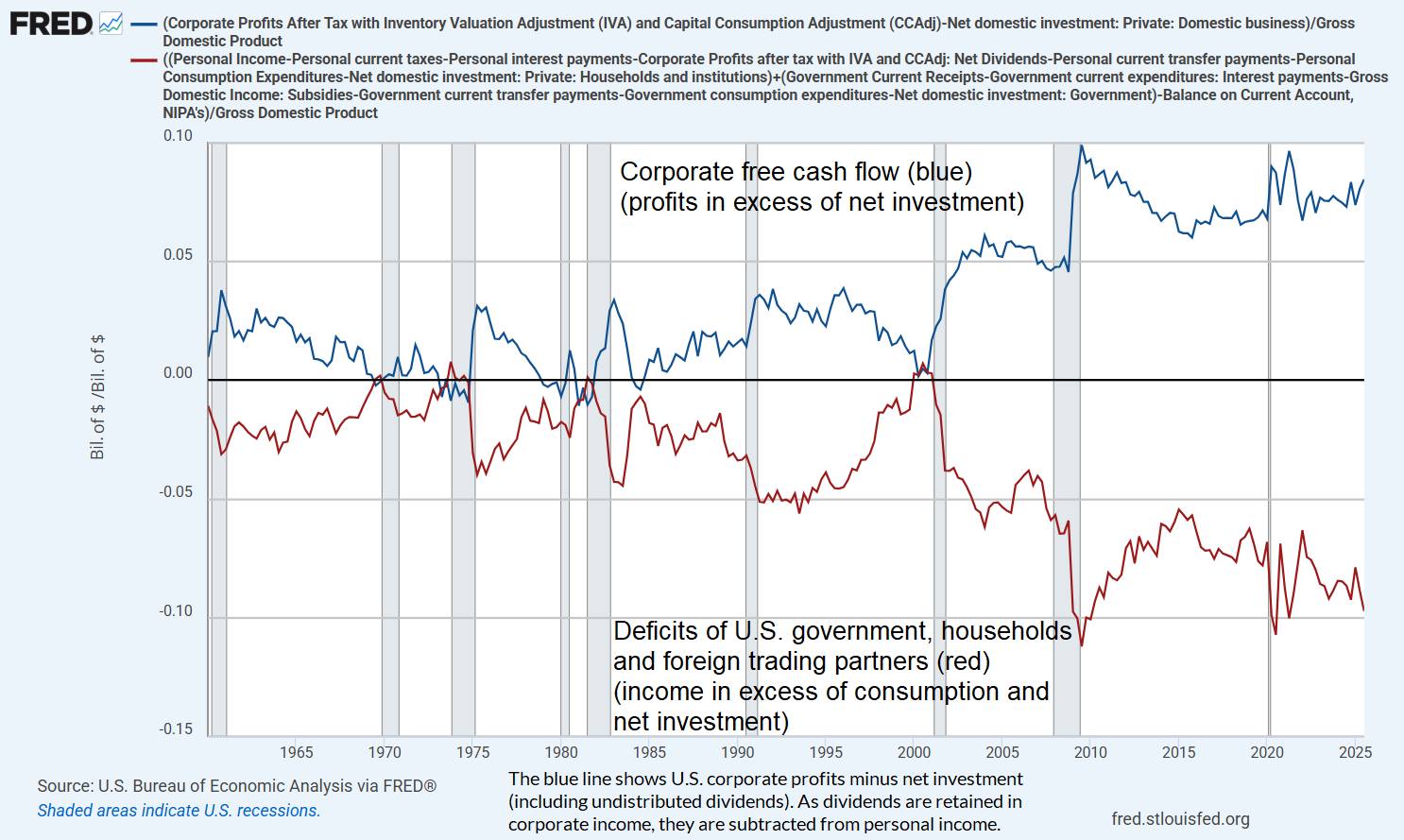
Given that the wealthiest 10% of U.S. households hold 87% of U.S. equities and mutual fund shares, 87% of loan assets (indirectly via claims on banks and other intermediaries), and 79% of debt securities (Data: Federal Reserve Distributional Financial Accounts), this trajectory illustrates the increasingly lopsided equilibrium in the U.S. economy: we see ordinary households struggling, with wage and salary income at the lowest share of GDP in history, while corporate profits and the wealth share of the top 10%, 1%, and 0.01% of households stands at unprecedented extremes.

Yes, it’s an equilibrium, but it’s a bonkers equilibrium. And it is also a policy choice. The simple fact is the corporate profits and financial gains – new income, new money, new wealth to the receivers – are taxed at wildly lower combined rates than wages and salaries. Indeed, many of the wealthiest households receive most of their compensation in stock, with the dilution offset by corporate stock buybacks (which avoids being taxed as dividends). They borrow against that stock in order to consume, while the gains can be deferred almost forever, making the present discounted value of the future tax liability close to zero.

There’s an argument that a low tax on financial “capital” (stocks and bonds) encourages productive investment (physical investment – the “I” in the GDP equation), but this is a terribly indirect way of doing it. It would be more efficient and less distorting to equalize combined tax rates between wages and salary income and financial income, while broadening the payroll tax base, lowering payroll tax rates, and using investment tax credits and accelerated depreciation to sustain real, productive investment directly.

By equalizing “combined tax rates”, I mean the combined impact of corporate taxes and taxes on the resulting investment returns (dividends + capital gains) on one hand, and the combined impact of income taxes on wages and salaries and the associated payroll taxes on the other. You remove the distortion by taxing a dollar of income as a dollar of income regardless of source, rather than skewing the code against wage and salary income. Broadening the base also allows you to lower the rates. You directly encourage investment and innovation, well, by encouraging it directly.

Meanwhile, we continue to see massive “natural monopolies” – companies that benefit from network effects and hyperscale (an uncompensated public good created by the very customers that act as hubs in the network). Similarly, tools like AI can be remarkably useful, but they are built by scouring the publicly available work, research and writing of countless people who go uncompensated, and the role of these technologies in improving productivity can come at the cost of displacing workers. These individuals still have to eat, support their families, retirement, and get health care, so they issue liabilities, or receive transfer payments funded by government liabilities, all of which are accumulated by households at the top of the income distribution.

Here, my own proposal would lean toward taxing the portion of corporate receipts that behave as “dominance rents” without fostering either employment or investment. An example of that definition would be gross value added, minus a per-worker allowance for wages paid (capped at, say, $150k each), minus a normal return allowance (a common benchmark return times the company’s actual base of real capital investment and R&D). This way, even if all human work is eventually replaced by a single corporation’s self-replicating AI robot toasters, humanity will not be in the position of borrowing from the one guy who owns the company, in order to consume the output generated by that company.

All of this is a choice. When you give a tax preference to a given activity or form of income, you get more of it, and that includes extreme wealth. When you create a tax disincentive, you get less of it, and that includes wage and salaries of working families. The point here isn’t to disparage anyone, only to observe that this is, because that is. We can certainly make policy choices that treat a dollar of income as a dollar of income, regardless of the source, while still encouraging productive investment, capital formation, jobs, and innovation.

We can understand the underlying condition of the U.S. economy only if we understand the equilibrium that we’ve allowed and even encouraged in recent decades.

Total income and total output are equal, but distributed in wildly different ways

There are two ways to calculate Gross Domestic Product (GDP) – the value of the nation’s economic output. One way is to add up the value of all goods and services that are produced by the economy (whether those goods and services are used for consumption, capital investment, or even unintended and unsold inventory). The other way is to add up all of the income received by every sector of the economy, including consumers, businesses, government, and in an open economy, foreign trading partners who sell us goods and services. Apart from a small “statistical discrepancy,” these two definitions of economic activity – the output and income definitions – are equivalent.

Suppose that working families help to produce the total output of the economy, but their wages and salaries fall short of the amount that they actually need in order to finance their consumption, living needs, health care, and retirement expenses. Well, for these families (about 90% of American citizens), their spending on consumption and net investment will be greater than their income. They finance that shortfall either by issuing liabilities directly (consumer loans, credit card debt, mortgage obligations), or by receiving government funds (social security, medicare, medicaid, SNAP, and other transfers, which amount to about two-thirds of all Federal spending). If government runs a deficit, it finances those transfers by issuing its own liabilities, as Treasury securities and monetary instruments.

It must then be true, in equilibrium, that the remaining sectors have received income above and beyond what they spent on consumption and net investment. Why? Because under the two identical definitions of GDP, total income is equal to total output (consumption and net investment, including inventories, whether intended or unintended). If one sector runs a shortfall, the others must run a mirror-image surplus.

As we saw in the January comment, the result over the past two decades is that the wealthiest 10% of American households have persistently accumulated an enormous amount of “savings” – which primarily take the form of newly issued liabilities of government and 90% of U.S. households. The U.S. economy is quite literally balanced on the back of working families and the Federal transfer payments that bridge the gap between household income and spending.

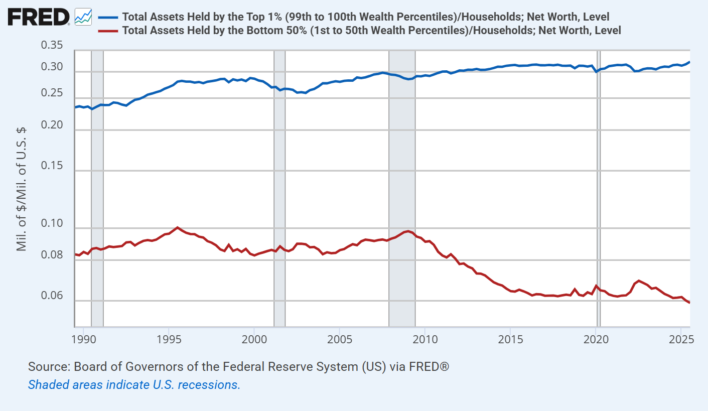
The chart below shows the total assets of the top 1% of U.S. households, compared with the bottom 50% of U.S. households, both as a ratio of total U.S. household net worth.

When we look carefully at the interconnectedness of things, we discover that the new “savings” in the U.S. economy always take the form of financial instruments that someone issued in order to finance mirror-image “deficits”. Although these new instruments may include newly issued shares of stock, the fact is that net issuance of U.S. stocks has actually been slightly negative over the past 20 years, meaning that “new savings” haven’t taken the form of stock shares.

Since 2000, the increase in U.S. stock market capitalization has been driven almost entirely by two factors: growth in fundamentals and, far more importantly, rising valuation multiples – not by the creation of new shares. What has increased dramatically is the outstanding debt of households and government. It has increased because our policy choices tolerate and even encourage a dramatic income skew between haves and the have-nots. This is because that is. This is not because that is not.

The deficit of one sector emerges as the surplus of other sectors, and the liabilities issued by one sector become the assets of the other sectors. It’s not just a theory. It’s an accounting identity.

Yes, corporate profits and free cash flow are at record highs. They’re at record highs because government, households and foreign trading partners are running a massive net deficit. The distribution of the corporate profits absolutely reflects scarcity, innovation and – particularly in recent years – “hyperscale” network effects, where single companies operate as dominant providers in their sectors. The level of profits, however, is a sectoral imbalance.

This enormous domestic imbalance between “haves” and “have nots” means that the “haves” accumulate the financial obligations of the “have nots.” That’s how this house of cards keeps standing.

Neither the government nor the average American household is taking in enough income to meet their expenditures. The majority of Federal expenditures are an offset to the fact that U.S. households, in aggregate, don’t earn enough to finance basic needs like healthcare and retirement expenditures. To a large extent, the combined deficit reflects a single underlying dynamic. From an accounting standpoint, record corporate profits are the mirror image of that dynamic.

– John P. Hussman, Ph.D., An Unstable Equilibrium, October 28, 2025

Objective functions

Whenever we talk about “maximizing” something, whether profits, or GDP, or expected returns, or the well-being of ourselves, our communities, or the world, we implicitly or explicitly create an “objective function” that takes certain inputs, like X1, X2 and so on, and converts them into the resulting thing, Y, that will make us happy, and that we want to maximize:

Y = function(X1,X2, …)

We should be careful about how we create our objective functions, for two reasons. One is that whatever we don’t include in our definition of happiness, and give zero weight, will be treated only as a means to our own happiness. We may then exploit or even destroy those things as long as they contribute to our pursuit. That leads to the second reason we need to be careful: there are often unobserved “feedback effects” from one variable to another. If we choose our objective function carelessly, we can actually harm ourselves.

Suppose we want our portfolios to earn high yields over time. We might decide to construct a portfolio made only of high yield securities, not realizing that by maximizing yield alone, we may also maximize the risk of bankruptcy and credit default. If we’re farmers, we might choose to maximize a harvest by bathing our crops in insecticide, inadvertently poisoning both the land, and our bounty of fruit.

The same is true in our daily lives and in our world. If our objective function gives full weight to our own wealth and happiness, and zero weight to the well-being of others, we may create a world where people in our own country and vulnerable populations elsewhere are exploited and discarded as “resources” that contribute to our profit. We might even poison the water we drink, the air we breathe, and the single planet in the cosmos that’s inherently symbiotic with humanity. In that case, our happiness may be made of the suffering of others, and that of our children and grandchildren. There may also be feedback effects – we may see homelessness, poverty, addiction, and social problems around us, without realizing that this is, because that is.

We may see people trying to escape from their condition and enter the U.S., seeking to share in some of our happiness, and we may turn them into enemies without realizing how our choice of objective function has contributed to the situation, or might be changed in ways that alleviate it. If the suffering and desperation of others hardens, we may even see crime, or violence, or hatred directed toward us. None of those things are born whole. They emerge because they are cultivated, sometimes intentionally, and sometimes inadvertently.

Either way, it helps to be aware of what we’ve included in our objective function, and to ask whether we’ve considered the feedbacks. If equilibrium teaches us one thing, it’s that nothing exists by itself alone.

Back to equilibrium in finance, we’ll next ask the question – why do prices change in the financial markets? This will give us a clean and exhaustive set of places to look, which taken together must account for those price changes, by definition.

We’ll then take a look at equilibrium in the stock market – the effect of investors who care about expected returns and risk, and price-insensitive investors who don’t. By the end of this comment, my hope is that it will be clear how such “flows” between buyers and sellers affect the financial markets.

Finally, we’ll examine the “bubble on a bubble” that we’ve observed in the information technology sector, and show the basic condition – “perceived edge” – that largely accounts for the huge share of market capitalization that these companies presently comprise.

The dentist in Poughkeepsie

Why do security prices fluctuate? What moves the market? Is it trading volume, “money flow”, fundamentals, changes in the expectations of investors about return and risk, or some combination?

The answer is that price fluctuations can be equally described in two seemingly different ways. At the base, the price of a given security is whatever the current perceptions, expectations, exuberance, hopes, and fears of buyers and sellers collectively determine the price to be. There’s no stable linear relationship between observable facts and prices. There isn’t even a stable nonlinear relationship. However, once investors collectively determine the price of a security, there is a very robust relationship – sheer arithmetic – that links three objects: the price investors pay, the very long-term stream of cash flows the security will deliver into the hands of investors over time, and the long-term rate of return that investors will enjoy or suffer if they buy the security at the current price.

Let’s begin with an observation about “equilibrium.” If a dentist in Poughkeepsie sells a single share of AAPL at a price that’s 7 cents below the previous trade, a billion dollars of market capitalization vanishes – a billion dollars, on $260 bucks of “flow.” Market capitalization is the outstanding number of shares times price, and price will move to whatever level that’s needed to ensure that someone holds every outstanding share. The marginal investor prices the whole float.

Intuitively, even though our dentist sells only a single share of AAPL, one could argue that other investors wouldn’t allow the stock to drop by even 7 cents unless the most eager buyer got just a bit less eager. That intuition is exactly right. What allows $260 bucks to move the market by a billion dollars is, implicitly, that other investors essentially agree that the price should be 7 cents lower. If some news event changes the collective view of investors about expected returns or expected risk, price can advance or decline sharply on very little volume.

Technically, all that’s needed to wipe out that billion dollars is for bids and offers to change. Once these quotations establish the neighborhood, trading a single share is enough to set the price. At the moment a trade occurs, there’s one price that results in everyone in the market holding every outstanding share of AAPL, and in this case, it’s 7 cents lower than the previous trade.

We can equivalently think about the price movement from the perspective of the arithmetic that links valuations and expected returns. The price change in AAPL tells us one of two things: either the market’s collective expectations for the future cash flows of AAPL have just declined by a tiny bit, or the long-term return that can be expected by the remaining holders of AAPL just increased by a tiny bit. That’s how valuation arithmetic works. One might say that a market where $260 bucks can move market cap by a billion dollars is wildly “inelastic,” but what’s actually going on is that the consensus view of investors has changed a tiny bit.

If a dentist in Poughkeepsie sells a single share of AAPL at a price that’s 7 cents below the previous trade, a billion dollars of market capitalization vanishes – a billion dollars, on $260 bucks of ‘flow.’ Market capitalization is the outstanding number of shares times price, and price will move to whatever level that’s needed to ensure that someone holds every outstanding share. The marginal investor prices the whole float.

It’s sometimes convenient to break the long-term expected return of a security into the sum of a “risk-free” rate and a “risk premium.” That decomposition is conceptual, not an assertion that investors actually do these calculations, but it does allow us to break price fluctuations into exactly three components:

1) Changes in the present level and expected trajectory of fundamentals,
2) The level of return available on competing assets (e.g. interest rates), and
3) Changes in the amount of compensation that investors require for accepting risk – which depends heavily on their psychology toward speculation or risk-aversion at any given time.

A financial “security” is nothing more than a claim on some stream of cash flows that investors expect to be delivered into their hands in the future. For any stream of future cash flows, and some long-term rate of expected return, we can always calculate the “present value” of the cash flows expected at each point in the future. If the price we pay today is the same as that “present value,” and the expected future cash flows actually emerge, our actual long-term investment return – by definition – will be exactly the long-term rate of return we used to discount the cash flows. For more discussion on this relationship, see the first half of How The Bubble Manipulates Time.

If you consider a world where record government and household deficits have emerged as mirror image corporate profits, while more than a decade of zero interest rates, coupled with speculative exuberance, encouraged investors to drive discount rates and risk-premiums to the lowest levels in history, you can understand why U.S. stock market valuations are at the most extreme levels in history. The problem is that understanding isn’t the same thing as justifying. Current valuation extremes now rely on those government and household deficits to continue forever. Meanwhile, the record low discount rates – reflected in historically extreme valuations – also imply the likelihood of meager long-term stock market returns even if expected cash flows are realized.

The chart below shows our most reliable gauge of market valuations in data since 1928: the ratio of nonfinancial market capitalization to gross value-added (MarketCap/GVA). Gross value-added is the sum of corporate revenues generated incrementally at each stage of production, so MarketCap/GVA might be reasonably be viewed as an economy-wide, apples-to-apples price/revenue multiple for U.S. nonfinancial corporations.

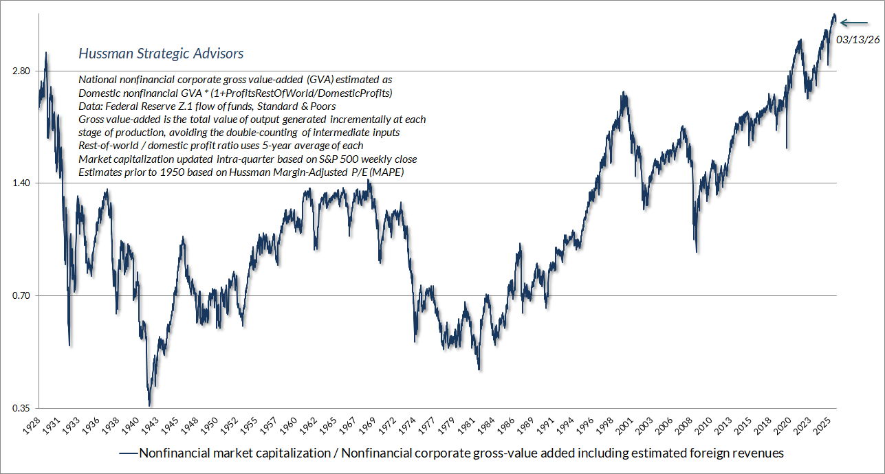
As I noted in January, over shorter horizons, all that matters is the return in people’s heads. It’s only over time that the cash flows arrive and reliably teach investors that valuations matter. That’s why Ben Graham wrote “In the short run, the market is a voting machine, but in the long run, it is a weighing machine.”

Current market conditions

The way to wealth in a bull market is debt. The way to oblivion in a bear market is also debt, and nobody rings a bell.

– James Grant

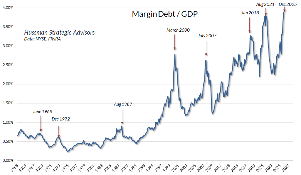
Among the recognizable features of speculative exuberance in recent months is the expansion of margin debt in investor portfolios. As I’ve noted many times over the years, one can normalize margin debt based on a variety of denominators, some more informative than others. For example, it’s tempting to normalize margin debt against market capitalization, but part of the information signal in margin debt is actually valuation, so you’re better off normalizing against measures that are more directly related to cash flows.

The chart below shows the ratio of margin debt to GDP. What matters for this particular measure isn’t the specific level, but the very discrete “spikes” – these tell you something about herd exuberance. My impression is that much of the recent spike is focused on information technology stocks. Historically, these spikes have added a layer of “forced selling” onto the market losses of speculative glamour stocks, as we’ve seen in other episodes. Like many indicators, Margin debt / GDP is best used as part of a broader set of information. The spike we see at present isn’t a powerful indicator in itself, but it does reinforce the signals we see in other areas, particularly valuations.

The overall condition of the U.S. stock market continues to feature near-record valuations and ragged internals. Still, particularly since our September 2024 hedging implementation, shorter-term market behavior can provide numerous opportunities to vary the “intensity” of our hedge, and as I noted last month, we’ve extended that implementation to identify conditions where we can even periodically reverse the hedge to a more constructive position – although unquestionably with a safety net at current valuation extremes. Suffice it to say that while the full-cycle implications of current valuations are still quite unfavorable, but we have no reliance on short-term forecasts or scenarios, since even the tilt of our own investment outlook can change from day-to-day and week-to-week as market conditions evolve.

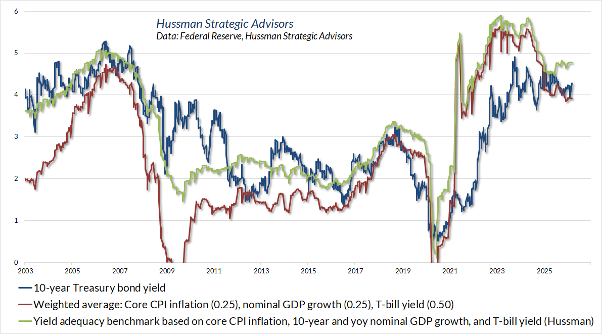
On the subject of debt, Treasury yields have pushed higher in recent weeks, partly in response to concerns about oil prices and prospects for higher government spending and faltering foreign demand for U.S. debt obligations. Even our simpler gauges of yield adequacy suggest that Treasury bond yields remain “meh” – not clearly inadequate, but not at levels where we’ve typically seen Treasury bonds returns reliably outpace T-bill returns. Overall, our bond market view is tepid here, but I expect that will gradually improve if we see a further push higher in yields.

Meanwhile, given that the entire total return of the Philadelphia Gold & Silver Index (XAU) has historically accrued during periods of falling bond yields, gold stocks have not surprisingly struggled amid a combination of rising yields and slightly improved readings from purchasing managers surveys and the like. These conditions will change, but presently our view on the sector is also rather tepid.

A simple valuation model

Getting back to the relationship between stock prices, fundamentals, and the expected returns in the heads of investors, let’s relate prices, cash flows, and expected returns so we can see very clearly what drives market fluctuations. Again, if math gives you hives, feel free to read around it – the math is here to provide structure and avoid the mud of purely verbal arguments.

By convention, I usually write future cash payments as C or D. Beyond that, we don’t need to restrict ourselves to the form that those cash payments will take. They can be dividends, lump sum buyout proceeds, extraordinary distributions, whatever. For modeling purposes, it’s often simplest to model the cash flows as growing smoothly over time at some rate g – but even here, we don’t need to restrict ourselves to a constant growth rate, or two stages of growth, or even a smooth path for growth rates over time. Simple models can provide enormous insight – we needn’t take our simplifying assumptions literally.

Price fluctuations break into exactly three components:
1) Changes in the present level and expected trajectory of fundamentals,
2) The level of return available on competing assets (e.g. interest rates), and
3) Changes in the amount of compensation that investors require for accepting risk – which depends heavily on their psychology toward speculation or risk-aversion at any given time.

With that in mind, suppose we’ve got a stock or other security. Let the price at any point in time be \(P_t\). Our security is expected to deliver some stream of future cash flows \(D_t\) to investors over time.

We’re particularly interested in our long-term expected rate of return – call it \(k\). That rate of return is the “slope of the line” between present and future. For example, if \(k\) is 10%, we expect $1 today to grow to $1.10 a year from now. Conversely, if we expect $1.10 a year from now, its “present value” is $1.10/(1.10) = $1.

Suppose investors use the rate of return \(k\) to discount expected future cash flows to present value, and buy the security at that price. If the expected cash flows actually materialize, then investors will actually earn \(k\) as their long-term return. For instance, suppose an IOU promises to deliver $100 a decade from today, and you pay $100/(1.08)^10 = $46.32 for it today. If the security actually delivers the expected $100 a decade from today, you will have earned an average annual return of ($100/$46.32)^(1/10)-1 = 8%.

In contrast, if the “psychological” expected return in investors heads, say \(k_h\) is different from the “fundamental” long-term rate of return \(k_f\) that equates the current price with discounted future cash flows, then it’s likely that reality will close that gap. For example, suppose that – based on past history – you simply assume that “IOU’s have an 8% return” and, confident in that 8% expected return, you buy the IOU today for $122. Well, regardless of the 8% expected return in your head, the price you paid ensures a -2% annual loss on the security over the coming decade. Now, that doesn’t mean you won’t be able to find a greater fool to take it off your hands at an even higher price between now and then, but for that investor, the consequences will be even worse.

For now, we’ll use \(k\) generically. If the “risk free” return \(R_f\) is the expected annual return from investing in a continuous sequence of short-term T-bills or other safe assets, we can write \(k\) as the sum of that risk-free rate \(R_f\) plus a “risk-premium” \( \zeta \) which compensates the investor for whatever risks they aren’t willing to accept for free.

Many of the risks that investors care about – uncertainty about future cash flows, interest rate volatility, default risk – have nothing to do with the trading behavior of other investors. We’ll call these “baseline” risks. Investors who care about expected return and risk will demand compensation for these risks. That’s true even if a single price-sensitive investor is needed even to hold a single share. Because every share must be held in equilibrium, the “marginal” price-sensitive investor prices the whole float.

So we can conceptualize the “risk premium” of the market even further by breaking it into a “baseline” component plus a “liquidity” component. The baseline or fundamental component of the equity risk premium is the premium that would exist even in the absence of price-insensitive disturbances. The liquidity or position-bearing component is the additional premium required to induce price-sensitive investors to depart from their baseline position by taking the other side of the trades placed by price-insensitive investors

For example, there’s no question that large, abrupt block trades can move stock prices, particularly when they create short-term order imbalances. But that’s only one component of the price-determination process. Even without order imbalances, price movements are driven by a combination of changes in investor expectations about the level and trajectory of fundamentals, and changes in the expected returns that investors require (interest rate plus risk-premium) for the wide range of baseline risks they care about.

Now let’s create a valuation multiple. The most important feature of any good valuation multiple is that the fundamental you use should be representative and proportional to the possibly very long-term stream of cash flows investors can expect. For example, if earnings and profit margins fluctuate from year-to-year or even decade-to-decade, a single year of earnings is not a reliable fundamental. That’s why smoother fundamentals like revenues tend to be more useful if one wants to relate current valuations to future expected returns.

For simplicity, suppose our cash flows grow at some relatively smooth rate \(g\), and that the fundamental \(F_t\) we use for valuations is roughly proportional to expected cash flows, at least on average. If dividends are some fraction \(m\) of our fundamental, we can write \(D_t = m \,F_t\), and we can define a valuation multiple \(V_t = P_{t} / F_{t}\).

Finally, if we write the security price as the sum of expected future cash flows, and the growth rate \(g\) is smooth, the arithmetic simplifies significantly. The result has the same form of the “Gordon growth model”

\[
P_t = \frac{D_t}{k-g} = \frac{m \, F_t}{R_f \,+ \,\zeta \,– \, g }
\]

Other things equal, prices will grow as fundamentals \(F_t\) grow. The valuation multiple gauges the horse-race that results as prices and fundamentals change over time. Rearranging a bit, we can write valuations as:

\[
V_t = \frac{P_t}{F_t} = \frac{m}{R_f \, – g + \,\zeta}
\]

Look carefully at the various components of valuations. Since a larger denominator will reduce prices and valuations, we see that prices and valuations will fall if interest rates rise more than the growth rate of fundamentals rises, or if investors demand a larger risk-premium \( \zeta \) for whatever risks they aren’t willing to accept for free. Conversely, prices and valuations will rise if interest rates decline more than the growth rate of fundamentals declines, or if investors demand a smaller risk-premium \(\zeta\).

When investors are inclined to speculate, their expectations for the trajectory of future cash flows can be inflated, and they may require very little compensation for accepting risk. That combination is a recipe for elevated prices and valuations. In contrast, when investors are inclined toward risk-aversion, their expectations for the trajectory of future cash flows may be dismal, and they may require very high compensation for accepting risk. That combination is a recipe for depressed prices and valuations.

Prices and valuations will fall if interest rates rise more than the growth rate of fundamentals rises, or if investors demand a larger risk-premium for whatever risks they aren’t willing to accept for free. Conversely, prices and valuations will rise if interest rates decline more than the growth rate of fundamentals declines, or if investors accept a smaller risk-premium.

As I’ve detailed previously, higher valuations imply greater volatility in response to any change in the risk-premium and expected long-term return. Indeed, we can show mathematically that for small changes in expected return, the “duration” of the S&P 500 is essentially its price/dividend ratio. The estimate is most accurate for small changes. So, for example, if the S&P 500 price/dividend ratio is 40, and the dividend yield increases by 5 basis points, prices will drop by about 40 x 0.05 = 2%. For more on this, see the section titled “Valuations and investment duration” in How to Spot a Bubble.

This result is particularly useful for market indices where dividends generally track other fundamentals over time. Other methods are required for individual stocks that don’t pay dividends, or when current dividends are not representative or proportional to long-term stream of cash flows paid out by the security. On this point, S&P 500 index dividends are, in fact, adjusted to capture the effect of net buybacks, so price-dividend is a reasonable measure of price sensitivity and duration.

Presently, the price/dividend multiple of the S&P 500 stands at 80, near the highest level in history with the exception of March-September 2000, when the price/dividend multiple reached 93. Dividends are also higher today as a share of revenues than they were in 2000. If dividends were the same ratio of sales as they were in 2000, the current price/dividend multiple would be 134.

Suffice it to say, with the U.S. stock market near the lowest estimated risk-premium in U.S. financial history, even a very small increase in the long-term return demanded by investors could have a profoundly disruptive price impact. A market crash, after all, is nothing but risk-aversion meeting a market that’s not priced to tolerate risk.

Beliefs, fundamentals, and information

Back in the 1980’s, a lot of the research in finance focused on ideas like the “efficient markets hypothesis” – the idea that even if people had private information, the willingness of rational investors to buy or sell could be taken as a signal that they had favorable or unfavorable information, so prices would adjust to reflect that private information. In fact, you could go even further – if all traders in the market were rational, the bids and offers would adjust without any trades needing to take place.

It’s rarely noted that the “efficient markets hypothesis” goes hand-in-hand with something called a “no-trade theorem.” If all traders are rational, prices fluctuate because bids and offers change, but no trade actually takes place. The willingness to buy or sell immediately conveys information. Everyone knows that everyone knows this (it’s “common knowledge”). Milgrom and Stokey’s “Information, Trade, and Common Knowledge” (1982) is the classic paper on this.

When traders have different information, and there’s also “noise” in the form of uninformed traders, or traders who buy and sell based on month-to-month liquidity, we do see trading volume. Purely passive investment can be thought of as a version of this “noise.” Frankly, I’m convinced that even passive investors care about investment return and risk – it’s just that in a speculative bubble, they become confident that investment returns don’t depend on price or valuation, because the rear-view mirror tells them so.

We can model beliefs, information, noise, and price impact explicitly – in fact, my doctoral dissertation at Stanford, more than 30 years ago, captured this sort of dynamic.

When investors trade both on their own beliefs, and on their beliefs about other people’s beliefs, and everyone infers the beliefs of others from market behavior, while market behavior itself is driven by everyone’s beliefs, modeling the problem quickly becomes very complex, particularly when not all trading is rational or information-driven. In his General Theory, Keynes (1936) likened the financial markets to a contest devoted to “anticipating what average opinion expects the average opinion to be. And there are some, I believe, who practice the fourth, fifth, and higher degrees.”

For decades, economists attempted to model those fourth, fifth, and higher degrees by introducing additional variables at every degree. This approach quickly produces a beliefs-about-beliefs-about-beliefs hall of mirrors called an “infinite regress.”

It wasn’t until 1992 that the problem was solved, in a paper  titled “Market Efficiency and Inefficiency in Rational Expectations Equilibria: Dynamic Effects of Heterogeneous Information and Noise.” I published it in the Journal of Economic Dynamics and Control. The approach applied signal extraction methods and extended a “fixed point” method that my dissertation advisor, Thomas Sargent, had developed to study learning, beliefs and information in the context of economic fluctuations.

Although studying beliefs in the financial market requires different modeling than for economic fluctuations, the common element is that the beliefs of individuals generate real-world outcomes, which are observed by those same individuals, who use that information to form their beliefs. As a result, a rational-expectations equilibrium is a “fixed-point”: Beliefs = Outcomes(Beliefs). In the financial markets, the problem is complicated by the fact that in equilibrium, price depends on itself, so I extended the method to satisfy an additional set of fixed-point conditions simultaneously.

In a market where some investors ignore information – about valuations for example – prices can still fully reflect all information provided that these “noise” traders are observable. If not, the beliefs of even rational traders can differ, and price may no longer reflect all information. Excess profits are then available over time, both as compensation for trades that embed information into stock prices, and for trades that provide liquidity to the noise traders – for example, buying into overextended selling pressure and selling into overextended buying pressure.

Regardless of whether noise is considered a supply or a demand phenomenon, the key characteristic is that the net supply available to fully rational traders is a random variable. When noise is unobservable, rational traders are faced with the signal extraction problem of discerning whether a change in price is due to other rational traders acting on private information about fundamentals, or whether it is due to fluctuations in unobserved supply.

The existence of predictable excess returns in an equilibrium with rational traders seems a bit odd. There are two factors which drive inefficiency in the market considered here. The first, clearly, is the existence of noise, which forces rational traders to hold a randomly varying supply of the security. This unobservable variation confounds the inference problems faced by traders, and causes them to rely heavily on their own information signals.

The efficiency of the market in a rational expectations equilibrium is enforced by profit opportunities which exist in a stable neighborhood of that equilibrium. In a market where all traders are rational, no trader is able to profit from private information because price conveys a signal to other market participants. This result is extremely robust with respect to the quality and allocation of private information, but is quite fragile in the presence of unobserved variability of asset supply. This ‘noise’ complicates the inference problems of traders, resulting in a number of features consistent with empirical evidence on actual markets. These features include divergence of opinion, trading volume, mean reversion, dividend yield effects, and ‘excess’ volatility.

– Hussman, John P. (1993), Market Efficiency and Inefficiency in Rational Expectations Equilibria

In the actual financial markets, we observe a great deal of trading. On a typical day, over $1 trillion of market capitalization changes hands, about half on the U.S. stock exchanges, and the other half in off-exchange (dark pool) trading. That daily trading is close to the annual amount of total personal savings across every household in the nation. In the calendar year ended June 2025, a record $457 billion “flowed into” passive U.S. mutual funds and ETFs, which then used those funds to buy stock from other investors (the sellers, of course, received those funds). That $457 billion amounts to less than one day of average trading value on U.S. exchanges, and about 0.3% of annual trading.

There’s little relationship between this trading volume and the direction or absolute change in prices. If investors generally agree about the implications of new information, the market can move by a great deal on a run-of-the-mill amount of trading volume. The price change alone can be enough to clear the market, because once price has changed, nobody is inclined to actually change their investment position at the new price.

In a panic or mania, prices may have to move by a great deal to restore equilibrium. If the herd is insensitive to the prices they’re trying to trade at – or worse, if advancing prices make a manic herd even more optimistic or falling prices make a panicking herd even more fearful, then huge price changes may be needed to induce enough investors to take the other side of their trades.

At the level of an individual trade, the bid-ask spread creates a bit of compensation for the person who takes the other side of that trade, as an incentive for providing or absorbing stock. The resulting “trade impact” is often like punching a pillow. In order to buy “at the market” you have to pay up and “lift the offer” price at which a certain amount of shares are available. In order to sell “at the market” you have to accept a slight discount and “hit the bid” price at which someone is willing to take the shares off your hands. Your trade makes a “dent” in the price, but in a world of two-sided trading, the dent gradually flattens out like a pillow, unless information has changed, or market makers are skittish and require a lot of compensation for stepping in front of what might be a freight train.

Taken together, price movements are driven by changes in the level of fundamentals, the expectations that investors have in their heads about the trajectory of future cash flows, and the long-term returns and the risk-premiums that they expect, and embed into prices, at any given moment. All this stuff clanking around in their heads is subject to waves of speculative or risk-averse psychology, the baseline risks that they care about, and their willingness or unwillingness to take the other side of day-to-day order flow.

Over the short-run, price will be whatever investors decide it will be – there’s no assurance that the expected future returns investors carry around in their heads are consistent with anything close to the returns that are consistent with the valuations they are paying. I actually think that’s what’s going on in the U.S. markets. The expected returns in investors heads are vastly higher than the returns implied by likely future cash flows. As Graham observed, in the short-run the market is a voting machine. Only in the long-run does it reliably behave as a weighing machine.

Investment returns as compensation

Our investment discipline is heavily influenced by that core idea that – at least over the complete market cycle – excess returns in the market are compensation for trades that provide some kind of service to other investors. In the more than three decades since I published that finance paper, our stock selection discipline has performed beautifully relative to the S&P 500. That discipline is heavily focused on a) valuation, b) inferring the information and psychology of investors from prices and market behavior, and c) providing liquidity to other traders by, as my friend Linda Raschke puts it “feeding the ducks when they’re quacking.”

Our hedging discipline also did beautifully across decades of complete market cycles, until Ben Bernanke introduced a “singularity” into the markets with zero-interest rate policy after the global financial crisis. We had to vastly increase our emphasis on market internals (the signal extraction method we use to infer information and investor psychology from prices and market behavior).

In recent years, these distortions have been amplified by massive government deficits and inadequate revenue generation. Every deficit emerges as the surplus of another sector. Yet many investors don’t seem to understand that record corporate profits are the mirror image of record deficits in the government and household sectors. Instead, investors have assumed that these record profits are permanent and have applied record valuation multiples to those record profits – a historically tragic form of double-counting.

Only in the past year have I felt content that we’ve adapted our hedging approach to tolerate and even thrive despite the horrific distortions that have been introduced into the markets in recent years (and remain to be resolved, most likely in a distressing way).

In my view, the most significant compensation investors will obtain in the coming years will result from feeding the ducks here at record valuations, and pre-committing to the internal fortitude that will later be required to catch falling knives as this bubble devolves – though with safety nets during periods when market internals remain ragged and divergent.

The broad range of measures we’ve developed across four decades – valuations, market internals, and various measures of overextension – served us extremely well over prior complete cycles. I expect they’ll be useful over the completion of the present one. This particular bubble has gone beyond precedent. Emphatically, nothing in our discipline requires a collapse, but I do believe the highest compensation will come from being prepared, at least, for exactly that.

Strangeness adds to the weight of calamities, and every mortal feels the greater pain as a result of that which also brings surprise. Therefore, nothing ought to be unexpected by us. Our minds should be sent forward in advance to meet all problems, and we should consider, not what is accustomed to happen, but what can happen. For what is there in existence that Fortune, when she has so willed, does not drag down from the very height of its prosperity? And what is there that she does not more violently assail the more brilliantly it shines?

– Seneca, Moral Letters to Lucilius, 62-65 AD

Destroying long-term stability by chasing short-term comfort

As a side-note, among the things I’ve been grateful for in my academic life was to have a doctoral committee that included Thomas Sargent and Joseph Stiglitz – both Nobel laureates; Ronald McKinnon, who pioneered work on financial repression, particularly by central banks; John Taylor, another rational expectations theorist whose groundbreaking work in discretionary versus rules-based policy includes a heuristic – the Taylor Rule – that bears his name, and; Robert Hall, who was the longtime Chair of the NBER Business Cycle Dating Committee.

The Federal Reserve’s deranged foray into purely discretionary policy – taking interest rates to zero and the quantity of base money from 6% of GDP in 2008 (its historical norm) to 36% of GDP by January 2023 – was precisely the sort of financial repression, purely discretionary policy, and encouragement of malinvestment that destroys long-run economic stability and the ability of the financial markets to effectively allocate capital. The predictable result has been the third great speculative bubble in U.S. financial history, an economy with the widest wealth disparities on record, and behavior among both policymakers and market participants that’s become nearly indistinguishable from an episode of Jackass.

First, low interest rates encourage firms to invest in more capital-intensive technologies, resulting in demand for labor falling in the longer term, even as unemployment declines in the short term. Second, older people who depend on interest income, hurt further, cut their consumption more deeply than those who benefit — rich owners of equity — increase theirs, undermining aggregate demand today. Third, the perhaps irrational but widely documented search for yield implies that many investors will shift their portfolios toward riskier assets, exposing the economy to greater financial instability.

– Joseph Stiglitz, What’s wrong with negative interest rates?

In the case of more discretionary policy making, decisions are less predictable and more ad hoc, and they tend to focus on short-term fine-tuning. Policymakers show little interest in coming to agreement about an overall contingency strategy for setting the instruments of policy, and the historical paths for the instruments are not well described by stable algebraic relationships. The discretionary period included a massive housing boom and bust with excessive risk taking, a financial crisis, and a Great Recession whose depth was much greater than any recession in the Great Moderation period.

– John Taylor, Monetary Policy Rules Work and Discretion Doesn’t

In the financial markets, the most important warning sign of poor long-term investment outcomes is extreme valuation. In economics, the most important warnings come from distortions of price signals and quantitative magnitudes – interest rate distortions, large wealth disparities, enormous deficits, and monetary liabilities that become disconnected from GDP. It’s fair to say that taking the quantity of base money from 6% of GDP to 36% of GDP (currently about 22%) and keeping it there falls into the category of quantitative distortion.

Once investors and policy makers choose to ignore all the long-term warning signs, in return for the short-term comfort of kicking the can down the road – extending the distortions of the present in a way that makes the long-term consequences worse – all that’s left to do is buckle up and grab a tub of popcorn.

We don’t know how long current distortions will persist, and we’ve done an enormous amount of adaptation to remove any need for a return to historical valuation norms, or even any end to deranged policies. I suspect this bubble will end as all bubbles have ended, but it’s important to repeat that it’s enough for us for the market to fluctuate.

The “shall” that matters most in the Federal Reserve Act appears in Section 2A – a single paragraph: “The Board of Governors of the Federal Reserve System and the Federal Open Market Committee shall maintain long run growth of the monetary and credit aggregates commensurate with the economy’s long run potential to increase production …” That is the sole mandate of the Federal Reserve. It’s not a dual mandate. It’s a single mandate, and as the Fed adheres to that mandate, there are three outcomes the Fed is expected to pursue: “so as to promote effectively the goals of maximum employment, stable prices, and moderate long-term interest rates.”

To Jerome Powell’s credit, after initially extending the deranged policies of Ben Bernanke and Janet Yellen, he found his center, and he’s done a remarkably good job moving toward progressively more systematic policy. I was a rather stern critic of Powell’s early on, but it’s important to recognize that people can change, particularly when they’ve had the chance to demonstrate that change. As he leaves his role at the Federal Reserve, I think Powell has been a credit to the institution.

On insensitivity to valuations

When we examine the behavior of the stock market in recent years, there’s no question that investors have become increasingly insensitive, even dismissive, to valuations. This is nothing new. The progressive embrace of passive investment strategies has been a feature of every speculative bubble across history.

Conceptually, “price-insensitive” investors are market participants who exclude price (and by extension, valuations, and the expected returns implied by valuations) as a consideration in their holdings. For these investors, price adjustment is not an available way to change their demand, placing the burden of adjustment on other investors.

Over the past decade, the share of total U.S. stock market capitalization owned through equity mutual funds and ETFs has grown from about 25% to 34% at present. As a fraction of these assets under management (AUM), passive vehicles like index-funds have increased from less than 40% of AUM to more than 60% of AUM. As a result, the total share of U.S. market capitalization held in the form of passively managed mutual funds and ETFs has grown to 21%.

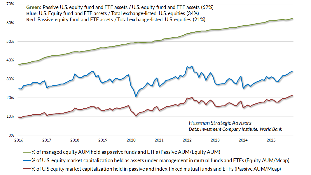
Now, the definition of a “passive” investment vehicle is a little bit squishy since, for example, many index-linked ETFs like the SPY, IWM and QQQ are actively traded.  Still, there’s no question that a larger portion of total equities is managed through passive vehicles.

It’s also conceptually squishy to equate “passive” investment with durable and reliable “price-insensitive” behavior. My impression is that all investors care about the long-term returns that they can expect from their investments. It’s just that long periods of market advance inspire a dangerous confidence that valuations have nothing to do with long-term returns. Instead, they come to imagine that long-term return prospects are always positive, and therefore that any price is a good price. If market history is clear on one point, it’s that this confidence can ultimately change on a dime.

Strictly speaking, there can be no such thing as an ‘investment issue’ in the absolute sense, i.e., implying that it remains an investment regardless of price. The ‘new era’ doctrine – that ‘good’ stocks were sound investments regardless of how high the price paid for them – was at bottom only a means of rationalizing under the title of ‘investment’ the well-nigh universal capitulation to the gambling fever. The notion that the desirability of a common stock was entirely independent of its price seems incredibly absurd. Yet the new-era theory led directly to this thesis… An alluring corollary of this principle was that making money in the stock market was now the easiest thing in the world. It was only necessary to buy ‘good’ stocks, regardless of price, and then to let nature take her upward course. The results of such a doctrine could not fail to be tragic.

– Benjamin Graham & David L. Dodd, Security Analysis, 1934

As I observed back in 2000 and more recently in The Bubble Term, the defining feature of a bubble is inconsistency between the expected returns in the heads of investors and expected returns based on valuations. The real issue in a bubble is always extrapolative expectations – the committed view of investors that stocks, or some sector of stocks, have a built-in “edge” regardless of valuation.

Rationalizing the bubble with “money flow”

Among the theories making the rounds these days, as “justifying theories” typically do during bubbles, is the idea that the financial markets are being buoyed by a constant “flow” of money “into” the market by price-insensitive investors.

There are two versions of the “flow” idea. The naïve one, repeated daily on financial television, conceives of the market as a bucket that money “goes into” when investors buy, and “comes out of” when investors sell. This notion is operating when news anchors talk about an up-day in the market by saying “investors put money into stocks,” and describe a down-day by saying “investors pulled money out of the market.”

The same notion takes the form of discussions about when the “cash on the sidelines” will finally “pour in.” What actually happens is that the dollars go “through” the stock market. The buyer’s cash goes to a seller. The seller’s stock goes to the buyer. A stock exchange is a place where shares of stock are exchanged. That’s why it’s called a stock exchange.

The trading that occurs in the stock market, as well as the so called “money flow” into and out of mutual funds and ETFs, is a reallocation of existing shares between different investors. The market is emphatically not a “bucket” or “balloon” or “jar” into which money flows, or whatever analogy one wishes to use. Not one dollar comes “off the sidelines.” A dollar is already a financial instrument in its own right. Net flow is zero.

If we say $1 billion “flowed” into equity mutual funds and ETFs, it means that investors transferred that amount to equity funds. The funds, in turn, create new fund shares, which are owned by the investor, and the cash is used to buy stocks. That cash goes to whoever sold that stock. We know that since about 2004, net equity issuance has been negative, as a result of corporate stock buybacks that have slightly exceeded new issuance. As a result of the new fund subscriptions, more shares are held by funds and ETFs, and fewer shares are held in the form of individual accounts and the like. It’s a change in ownership. The market isn’t a bucket, jar, or balloon (even if valuations are a “bubble”).

Yes, market capitalizations have changed over time, as a combination of growth in fundamentals and record speculative valuations, but investor savings aren’t going “into” the stock market month after month. As we’ve seen, the deficit of the government and 90% of households emerge as the “surplus” of corporations and 10% of households. In equilibrium, the surpluses (income in excess of consumption and net investment) take the form of whatever new liabilities – primarily government debt, base money, consumer debt, and mortgage debt – were issued to finance the deficits (consumption and net investment in excess of income).

A second, more sophisticated view of “flow” – and one that has a kernel of truth, is the idea that investors have increasingly embraced passive investment strategies. This observation has increasingly been extended to an argument that markets are dominated by price-insensitive “flows” that drive prices ever higher because the markets are “inelastic.” It’s also argued that these “flows” are driving large-capitalization stocks to progressively larger market capitalizations and index weightings; and that they will continue to buoy the market, possibly indefinitely, but in any case, until the flows stop flowing.

There’s certainly ground for agreement on certain points. After a very extended market advance, with fiscal and monetary stick-saves after every decline, investors have clearly developed a sense of certainty that “the market always comes back,” embracing the doctrine that, in the words of Graham and Dodd, it is “only necessary to buy ‘good stocks,’ regardless of price, and then to let nature take her upward course.”

To the extent that passive investors are price-insensitive at this moment, my impression is passive strategies are only one of scores of “noise trading” influences operating in the markets, as one can discover by accidentally un-muting the volume on financial TV. Indeed, Robin Hood alone accounts for more equity trading value in a typical month than all new subscriptions into passive U.S. equity funds and ETFs combined. These broader sources of “noise” are two-sided, often with short or intermediate-term horizons. It’s difficult to characterize the daily frenzy of market activity as anything close to an unstoppable freight-train of long-term, passive buying.

It’s clear that order imbalances can move prices around, but there’s also a significant amount of price movement that’s not “forced” by trading. It’s driven by the expectations in the heads of investors. The market risk-premium can vanish in a bubble – not because of mechanical buying, but because the expected return in investors heads becomes misaligned with the long-term return that equates discounted cash flows with the market price.

My concern is that many investors have equated the prevailing confidence in an ever-rewarding market – a feature of every speculative bubble in history – with the idea that “passive flows” are the primary mechanism that has driven prices and valuations to record extremes, and prospective future returns to dismally low levels. Indeed, many seem to be appealing to the notion of “flows” as a justification for why this bubble will continue indefinitely.

This basic “passive flows” idea is reflected in a social media post that circulated late last year:

“Every dollar flowing into an S&P 500 ETF automatically allocates thirty-five cents to seven stocks. Not because someone studied the balance sheets. Because that is their index weight. Passive buying increases prices. Higher prices increase index weights. Higher weights attract more passive buying. The feedback loop operates completely independent of whether any business is worth what the market claims. The marginal buyer of American equities is no longer an analyst with conviction. It is a target date fund receiving its biweekly paycheck allocation. This buyer has no opinion. This buyer will never sell. Price discovery, the mechanism that has allocated capital for two centuries, has been structurally disabled.”

Easy now.

I detailed my impressions of this argument back in January, but because investors continue to ask about it, it may be helpful to reiterate those impressions.

The idea that the accumulation of outstanding shares by price-insensitive investors can drive “risk-premiums” lower, and therefore drive prices higher, is consistent with even my own academic research decades ago (e.g. Market efficiency and inefficiency in rational expectations equilibria: dynamic effects of heterogenous information and noise, Journal of Economic Dynamics & Control, 1992).

The problem is that in order to convert this idea into a theory of bubbles and permanent price impact, one needs to take literally the idea that a progressively increasing fraction of outstanding shares is held by investors who honestly do not care about expected returns or risk-premiums – and remain indifferent even to enormous cumulative reductions in likely future returns.

In effect, you’re assuming that price insensitivity applies not only to the marginal transaction (the order “fill”) but to the entire investment position. Given that assumption, and holding all other things equal, equilibrium implies that valuations are an increasing function of the holdings of passive investors. But this means – equivalently – that the holdings of passive investors progressively increase as their expected future returns decline, and that passive investors are just fine with that. The reason this poses no obstacle to equilibrium is because we’ve assumed that passive investors don’t care about expected returns – durably, and with respect to their entire position.

In the language of my 1993 paper, the “flows” argument implies that an increasing portion of the total float is held by “noise traders.” Expected returns simply don’t enter their “objective function,” so valuations have no impact on their desired holdings. While this is clearly a reasonable specification for, say, an individual “market order,” it’s difficult to extend it to the entire position – to assume that the marginal buyer is someone who keeps adding to their holdings despite increasingly thin return prospects, that they fully recognize are dismal. As I noted in January, this sort of equilibrium essentially sees passive investors as pod-people in the Invasion of the Body Snatchers. I don’t believe that for a second.

To be clear, there’s no question that institutional trading and order imbalances can have day-to-day price impact. But that’s different from saying that investors don’t care about prospective returns – that they’re perfectly content with progressively higher valuations and progressively lower expected returns. In my own view, the defining feature of a bubble is that investors come to believe stocks have a persistent “edge” that ensures attractive expected returns regardless of valuations, so prices impose no discipline on their behavior. This is a much more vulnerable equilibrium, because it requires only a psychological realignment of expectations to produce a market collapse.

In this way, my own argument is much more aligned with Graham & Dodd’s 1934 description of the market conditions that preceded the collapse of the Great Depression. They observed that long periods of market advance inspire a dangerous confidence that valuations have nothing to do with long-term returns. Instead, investors come to imagine that long-term return prospects are always positive, and therefore that any price is a good price. This is a dynamic that plays out in every bubble – it’s nothing new. Passive investing always becomes increasingly popular as a bubble proceeds.

This isn’t just semantics. If one views bubbles as Graham & Dodd did – that investors do care about likely future returns, but that their expectations are misaligned, then the idea of “flows” is dispensable because heterogeneity among traders isn’t required. A bubble requires only that consensus expectations about future returns are misaligned with the expected returns implied by fundamentals (see the Geek’s Note in The Bubble Term), a collapse requires only that the expected returns in the heads of investors become realigned with prevailing valuations.

In contrast, the idea that the bubble is driven by “price-insensitive money flow” seems to offer the additional assurance that there’s something mechanical and quantitatively decisive – about particular investors and the investment vehicles they hold – that supports stocks beyond speculative psychology itself. I believe that’s a dangerous notion because it encourages confidence that the bubble is “structural.”

In my view, the evidence is far more consistent with a world where valuations and sector weights are – for the moment – being driven by expectations for high future expected returns, regardless of valuations. In that world, it’s the expected returns in investors heads that support prices. But these expectations can change, as they have in every bubble throughout history.

If one views bubbles as Graham & Dodd did – that investors do care about likely future returns, but that their expectations are misaligned, then the idea of “flows” is dispensable because heterogeneity among traders isn’t required. A bubble requires only that consensus expectations about future returns are misaligned with the expected returns implied by fundamentals.

One might argue it doesn’t matter whether investors are “passive” because their views are overly optimistic, or because they’re legitimately price-insensitive. One might argue that these are observationally equivalent because both result in higher prices. The difference, however, is that the “flows” argument seems to promise the additional confidence that it’s the flows themselves, not investor psychology, that mechanically drive prices higher. It’s a subtle distinction, but the flows argument implicitly suggests that investors would need to divest their passive holdings in order for the bubble to collapse. Confidence that “this buyer will never sell” then equates to confidence that “prices will never decline.”

Again, I don’t believe that for a second. Expectations and prices can change without the need for large transaction volumes. Most of the day-to-day fluctuation in the market is driven by changes in information, investor expectations, and changes in speculative versus risk-averse psychology. The resulting price changes require no massive changes in the investment positions of the average investor. The marginal investor prices the whole float. Some portion of daily volatility undoubtedly represents premiums and discounts received by traders who take the other side of more price-insensitive trading, but that’s a component of the risk-premium, not the whole enchilada.

Even a dentist in Poughkeepsie is enough to move the market if consensus expectations have changed. It doesn’t matter if 21% of the float is held in the form of index-linked vehicles. If Martians colonize Earth over the weekend, or any vastly smaller event occurs that investors care about, the bids and asks will change because the expectations and risk-perceptions of market participants have changed. You don’t need order imbalances to push prices around.

The defining feature of a speculative bubble is that the expectations about future returns that investors carry around in their heads become disconnected from the prospective returns implied by valuations and properly-discounted cash flows. A bubble doesn’t rely on one-directional “money flow.” Rather, it relies on investors having expectations in their heads about future long-term returns, without adjusting those expectations lower as valuations increase.

The result is an ever-increasing gap between the long-term returns that investors imagine in their heads, and the long-term returns that are implied by, and are consistent with, valuations and discounted cash flows.

Put simply, I’m not at all convinced that price-insensitive “flows’ or mechanical “elasticity” are what’s driving current valuation extremes. I am, however, entirely convinced that investors have expectations about future returns in their heads that both encourage and reinforce passive investment strategies, and that these expectations about future returns have had a self-reinforcing impact on prices.

The vast majority of investors, in my view, are just as interested in future returns as value-conscious, price-sensitive investors are. It’s just that they’re also convinced that the future returns will be glorious. It’s not the mechanical quantity effect of their holdings – the share of outstanding stock they hold – that has driven prices higher. It’s the expectations in their heads. No significant amount of “selling” needs to occur in order for the house of cards to collapse. All that needs to happen is for expectations to be realigned. As with the collapse of any bubble, it’s not necessary for a huge proportion of investors to “sell”. What’s required is only that expectations and risk-preferences shift.

On the relationship between the “perceived edge” of a security and its optimal portfolio weight

Suppose investors can allocate investment funds across assets that provide risk-free interest, and a range of riskier securities that may be volatile, and possibly correlated with risks that the investor can’t diversify away. If we assume that investors care about expected return and risk, we can show how those expectations translate into the weights investors place on various securities.

The Geek’s Note at the end of this comment shows the most widely applied version of this model, which I used to teach my undergraduate students. The derivation involves maximizing the expected return of the portfolio, constraining expected volatility with a Lagrange multiplier (you know what I’m talkin’ bout, but now, I might be mistaken, a hmm hmm hmm, drum fill), taking first-order conditions, and then asking the key question:

“Under what condition does an investor choose to place no additional weight on any particular security beyond its weight in the market as a whole?”

The answer is this: the weight that investors place on any given security is a reflection of the risk-adjusted “edge” that they expect for that security.

Mathematically – skip this if you’re scratching your arms already – if the expected return of security A is \( E[R_a]\), the risk-free interest rate is \(R_f\) and the expected return of the market as a whole is \(E[R_m]\), the condition for “no overweight or underweight on security A” looks like this:

\[
E[R_a] = R_f + \beta E[R_m – Rf] \]

Where \(\beta\) is the sensitivity of security A to fluctuations in the overall market. Writing things in terms of expected risk-premiums \(\zeta_a = E[R_a – R_f]\) and \(\zeta_m = E[R_m – R_f]\), this reduces to

\[
\zeta_a = \beta \, \zeta_m
\]

An investor who is interested in maximizing expected return per unit of risk will overweight security A beyond its representation in the “market portfolio” if the expected risk premium provides an expected “edge,” given the exposure of that security to overall market fluctuations (\(\beta)\).

As investors, we shouldn’t expect to be compensated simply for taking risk itself. A poorly diversified portfolio, for example, may have more volatility and extreme returns, but it doesn’t have a higher expected return. Instead, the level of compensation (the “risk premium”) investors can expect depends on how correlated or uncorrelated the returns of that security are to market risks that the investor can’t diversify away.

That’s why investors often have an “alternative sleeve” in their portfolio allocations. A security that has a \(\beta\) of zero and an expected return even slightly above the T-bill rate can actually be used to improve the return/risk profile of the portfolio. Likewise, a security that has a negative \(\beta\) essentially acts as an insurance policy, and can improve the expected return/risk profile of the portfolio, versus an allocation between the market and cash alone, even if the expected return of security A is below the risk-free rate, and in some cases, even if the expected return of security A is negative, provided that the security acts as a buffer when things go wrong.

The concept of “perceived edge” is particularly helpful in understanding the bubble in technology stocks in recent years. To say that the weight on a particular stock, or set of stocks, is persistently rising in the market is to say that investors as a group believe that this stock or set of stocks has an “edge” that persists independent of valuation.

A bubble on a bubble

In the technology sector, my impression is that we’re in the late stages of a bubble on a bubble. Specifically, information technology stocks, particularly those that enjoy strong “network effects,” have enjoyed an amplified version of the dynamic I described in my August comment, The Bubble Term.

Emphatically, nothing in our investment discipline relies on a market collapse, or even any long-term reversion in market valuations – we’ve adapted enough to welcome even a bubble that never ends (see How I Learned to Love the Bubble). That allows us to be much more flexible, particularly provided we maintain a safety net, but it doesn’t mean we’ve let down our guard. I still suspect that the S&P 500 has a 60-70% market loss in its future over the completion of this cycle.

Consider some company A. The thing that will drive the market weight A higher and higher is the belief among investors that A has a persistent “edge” regardless of price. In that case, the price, market capitalization and index weight of A will advance, and in equilibrium, the extra return provided by A in this self-fulfilling bubble will be exactly the “edge” that investors imagine should exist. It’s not “money flow” that does the job. It’s this “perceived edge” that makes the weight increase.

From this perspective, it’s straightforward to explain a world where the index weights of individual stocks are “forced” higher. It’s a world where investors come to believe that certain stocks have a built-in performance edge, beyond the expected return of the market itself. I think that’s precisely the world we’re living in at the moment. It’s the shared belief in a performance edge that drives the stock’s market weighting higher. The prices are held up by preferences and expectations.

Nowhere is the “increasing weight” story more evident than in the technology sector. The chart below shows valuation of the S&P Information Technology index, based on price/revenue.

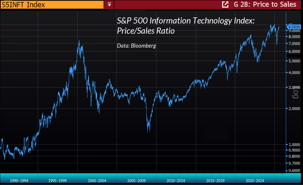
How do we know this trajectory isn’t just rational valuation at work? Well, one of the red flags is that, for the largest technology stocks, valuation multiples haven’t declined as enormous growth in fundamentals has proceeded. Despite profound revenue growth since 2000, many of the behemoths currently have price/revenue multiples close to or higher than the multiples they had in the late-1990’s.

Consider a company that’s expected to grow revenues and earnings at a very high rate over an extended period of time, before slowing toward the growth rate of the overall economy (we know that growth must eventually slow to a growth rate at or below the rate of economic growth, or the company would eventually represent 100% of GDP).

Well, unless investors collectively believe that the stock should provide a long-term return that’s even higher than the high-growth rate of fundamentals, valuation multiples should progressively decline during the high-growth phase. Suppose for example that fundamentals have doubled over the past year. Even if the stock was priced to provide 20% long-term annual returns, if price goes up by 20% as revenues and earnings double, the valuation multiple falls to 1.2/2.0 = 0.6 of what it was a year ago. As it should.

If valuations aren’t falling, one of two things (or both) must be occurring from a present-value perspective. Either there has been a significant decline in the long-term rate of return investors can expect, or investors are repeatedly shifting the entire trajectory of future growth higher – treating each period as a new starting point, but pushing the same high expected growth rate further and further into the future.

In my view, both of these are occurring. Specifically, valuations for the largest information technology companies are at levels that only make sense if one discounts optimistic future cash flows at depressed long-term rates of return. Meanwhile, these valuations suggest that the expected returns in the heads of investors are tethered to the current earnings and revenue growth rates of the companies themselves, as if these growth rates are permanent.

When investors think about the “edge” that a particular stock may have, it’s important to distinguish between an “edge” measured simply based on a backward-looking increase in price, and an “edge” based on a high expected future long-term investment return – driven by valuations that relate the current price with expected future cash flows. Often, investors imagine that stocks with very high past returns and explosive past growth in revenues and earnings obviously have an “edge” – believing that this past behavior frees them from having to examine valuations.

That’s the fatal error that investors commit in every speculative bubble. It’s exactly why we projected the scope for an 83% loss in technology stocks at the March 2020 market peak. From the 2000 peak to the October 2002 trough, the tech-heavy Nasdaq 100 followed just that trajectory – losing 50% of its value, followed by a loss of 50% of what remained, followed by the loss of nearly a third of what was left by the time the market bottomed.

Recall the largest three tech stocks at the end of 1999 by market capitalization: Microsoft, Cisco, and Intel. Their total returns, respectively, since 1999 have averaged 9.6%, 3.2%, and 2.6%. The average is 5.1%. Seeing the largest companies in each market cycle go on to lag, as a group, is the norm, not the exception.

As I observed in 2024 (see The Turtle and the Pendulum), high growth rates and profit margins aren’t fixed numbers. They’re trajectories. When investors value stocks based on extrapolation of the growth phase, they put a pendulum on their turtle and swing it all the way forward. The fact is that except during the speculative blowoffs that drive them to an extreme market share (e.g. 1929, 1972, 2000, today), the largest cap stocks tend to follow by underperforming the average stock over time.

Bubbles are generated when investors drive valuations higher without simultaneously adjusting expectations for future returns lower. In other words, the defining feature of a bubble is inconsistency between expected returns based on price behavior and expected returns based on valuations. The ‘Bubble Term’ measures the gap between the two.

Unless the Bubble Term is able to become exponentially larger forever – it shows up as a growing gap between the long-term return that investors expect in their heads, and the long-term return that investors can actually expect based on the future cash flows that will ultimately be delivered into their hands.

Sustaining the bubble requires valuation multiples to increase forever, without any upper bound. The reason the current bubble feels so good to investors is that, up until the present moment, valuation multiples have done exactly that.

– John P. Hussman, Ph.D, The Bubble Term, August 14, 2025

As Nobel laureate Franco Modigliani observed in March 2000, as the tech bubble was peaking, “The bubble is rational in a certain sense. The expectation of growth produces the growth, which confirms the expectation; people will buy it because it went up. But once you are convinced that it is not growing anymore, nobody wants to hold a stock because it is overvalued. Everybody wants to get out and it collapses, beyond the fundamentals.”

A few weeks earlier, on March 7, 2000, I observed “Over time, price/revenue ratios come back in line. Currently, that would require an 83% plunge in tech stocks (recall the 1969-70 tech massacre). If you understand values and market history, you know we’re not joking.” By October 2002, the tech-heavy Nasdaq 100 had lost precisely that amount of its market capitalization.

As valuations are driven higher, and true long-term expected returns – implied by discounted cash flows – are driven lower, my impression is that there is a widening gap between the expected returns that investors have in their heads and that actual returns that can be expected based on likely future cash flows. The effect is particularly amplified in the information technology sector.

The upshot is this. The U.S. equity markets stand at the most extreme point of valuation in U.S. financial market history. Record deficits in the government and household sectors have a mirror image that is observed as record corporate profits. While the distribution of these profits has benefited large technology companies that enjoy enormous network effects (a public good for which the public is not compensated), the level of these profits reflects a macroeconomic structure that taxes wage and salary income at vastly higher rates than it taxes income from securities and dividends, and leaves tens of trillions of dollars of capital gains wholly untaxed because they can be deferred without limit.

Meanwhile, investors have interpreted these profits as permanent, and are assigning record or near-record valuation multiples to these profits, generating a speculative bubble. At a sector level, the largest companies – particularly in information technology – are being priced as if they have a fixed “performance edge” regardless of valuations. This has produced a bubble upon a bubble, with a likely outcome not entirely different than the 2000-2002 collapse, in which the technology-heavy Nasdaq 100 index lost 83% of its value from peak-to-trough.

It stands repeating, again and again, that nothing in our investment discipline relies on a market collapse, or a long-term reversion in valuations. We’re certainly aware of the risks, and at current extremes, there’s no situation in which we would operate without a safety net against major market losses. At the same time, we’ve significantly adapted the implementation of our investment discipline – not only by increasing our ability to vary the intensity of “bearish” investment positions in September 2024 (see the section titled “The Martian” in The Turtle and the Pendulum) but more recently, by expanding our ability to periodically reverse our hedges from mildly bearish to “constructive with a safety net” – removing the “upside cap” on potential returns, even amid extreme valuations (see How I Learned to Love the Bubble).

I expect that my views will continue to sound “bearish” to the indiscriminate observer, because I write only once a month, and our hedging variations tend to be short-term in nature – even though they’ve allowed us to benefit from a generally rising market since September 2024, despite that generally “bearish” outlook. What’s important is to recognize that our views aren’t “forecasts” and we don’t require any particular market outcome. Our discipline is to consistently align our investment stance with objective, measurable, observable market conditions as they change over time. The best way to take good care of the future is to repeatedly take good care of the present moment.

Geek’s Note: Active investment weights reflect perceived “edge”

To provide some additional intuition on how investor perceptions are related to the active and passive weights that investors choose, here’s a derivation of a classic asset pricing approach that I used to teach my undergraduates at the University of Michigan. Emphatically, we don’t have to “believe” the “Capital Asset Pricing Model” itself. Rather, what’s important is the underlying concept: the weight that investors place on any given stock is a reflection of the risk-adjusted “edge” that they expect for that stock.

Suppose an investor can allocate investment funds across a risk-free investment earning \(R_f\), some individual stock \(A\) with uncertain return \(R_a\), the market portfolio \(M\) with uncertain return \(R_m\).

Define the portfolio weights on these assets as \(w_f, w_m, w_a\) with
\[
w_f + w_m + w_a = 1.
\]

The portfolio return can be written as

\[
R_p = R_f + w_a (R_a – R_f) + w_m (R_m – R_f).
\]

Its expected return is

\[
\mathbb{E}[R_p] = R_f
+ w_a \bigl(\mathbb{E}[R_a] – R_f\bigr)
+ w_m \bigl(\mathbb{E}[R_m] – R_f\bigr).
\]

Now consider the risk of the portfolio. Writing

\(\varepsilon_a = R_a – \mathbb{E}[R_a]\),

\(\varepsilon_m = R_m – \mathbb{E}[R_m]\),

and using \(\mathbb{E}[\varepsilon_a] = \mathbb{E}[\varepsilon_m] = 0\), the random part of the portfolio return (actual minus expected) is

\[
R_p – \mathbb{E}[R_p] = w_m \varepsilon_m + w_a \varepsilon_a,
\]

so the portfolio variance \( \mathrm{Var}(R_p) \) is

\[
\sigma_{p}^2  = w_a^2 \sigma_a^2 + w_m^2 \sigma_m^2 + 2 w_a w_m \sigma_{a,m},
\]

where

\(\sigma_a^2 = \mathrm{Var}(R_a)\),

\(\sigma_m^2 = \mathrm{Var}(R_m)\),

\(\sigma_{a,m} = \mathrm{Cov}(R_a, R_m)\).

Now suppose an investor chooses portfolio weights in order to maximize expected return for a given level of risk \(\bar{\sigma}^2\). We can write the Lagrangian

\[
\mathcal{L}  = \mathbb{E}[R_p] + \lambda \bigl(  \bar{\sigma}^2 – \mathrm{Var}(R_p) \bigr),
\]

with multiplier \(\lambda > 0\). Using our expressions for expected return and risk, taking derivatives with respect to \(w_a\) and \(w_m\), and setting them to zero gives these first-order conditions

\[
\mathbb{E}[R_a] – R_f
= \lambda \bigl(2 w_a \sigma_a^2 + 2 w_m \sigma_{a,m}\bigr),
\]

\[
\mathbb{E}[R_m] – R_f
= \lambda \bigl(2 w_m \sigma_m^2 + 2 w_a \sigma_{a,m}\bigr).
\]

The Lagrange multiplier \(\lambda\) reflects how much expected return the investor requires as compensation for a one-unit increase in portfolio variance.

You’ll sometimes see the investor’s “objective function” written as the problem of maximizing expected return minus a risk penalty: \(\gamma / 2 \) times portfolio variance, where \(\gamma\) is a measure of risk-aversion. That’s actually equivalent to our Lagrangian, and simply substitutes \( \lambda = \gamma/2\). The 2s that appear when taking the first derivative then vanish, leaving equations in \( \gamma \) alone.

Now, suppose we define the “market portfolio” broadly enough that every stock is represented. By definition, all stocks must be held – taking all investors together, their portfolio holdings will add up to “the market.” In equilibrium, this means that no stock can ever be “underowned’ or “overowned.”

Suppose, for simplicity, that investors share the same views about expected returns. What must be true about expected returns in order for investors to choose no additional active position in \(A\) beyond the weight it already has inside the market portfolio?

If the investor chooses \(w_a = 0\), the first-order conditions must reduce to

\[
\mathbb{E}[R_m] – R_f
= 2 \, \lambda \, w_m \sigma_m^2,
\qquad
\mathbb{E}[R_a] – R_f
= 2 \, \lambda \,  w_m \sigma_{a,m}.
\]

Eliminating the common factor \(2 \, \lambda w_m\) yields

\[
\frac{\mathbb{E}[R_a] – R_f}{\sigma_{a,m}}
=
\frac{\mathbb{E}[R_m] – R_f}{\sigma_m^2}.
\]

Finally, we can define \(\beta_A\) as the “beta” of stock A. For clarity, this is a different beta than the “bubble term” in my August 2025 comment, and in the Geek’s note that follows. Here, beta is defined as percentage change in stock A in response to a 1% change in the market. In other words, \(\beta_A \) measures how much market risk “loads” onto stock A. Statistically, \(\beta_A \) is defined as the covariance between the returns of stock A and the market, divided by the variance of market returns:

\[
\beta_A
= \frac{\mathrm{Cov}(R_a, R_m)}{\mathrm{Var}(R_m)}
= \frac{\sigma_{a,m}}{\sigma_m^2}.
\]

Substituting this definition of \(\beta_A\) into the optimality conditions, we find that the investor will choose not to hold any active weight in stock \(A\) – beyond its weight in the market portfolio – provided that the expected return of the stock precisely compensates the investor for the systematic, undiversifiable exposure to market risk “loaded” onto that stock:

\[
\mathbb{E}[R_a] = R_f + \beta_A \bigl(\mathbb{E}[R_m] – R_f\bigr).
\]

Defining the “risk premiums” of stock A and the market, respectively, as their expected returns over-and-above the risk-free rate, we can write this condition compactly as

\[
\mathbb{E}[R_a – Rf] = \beta_A \bigl(\mathbb{E}[R_m] – R_f\bigr)
\longrightarrow
\zeta_A = \beta_A \, \zeta_m.
\]

In short, investors will only “chase” stock A, beyond its weight in the market portfolio, if they believe stock A will provide them an “edge” – an expected return above the risk-premium one would normally expect based on the stock’s sensitivity to market risk itself.

If we add the equilibrium condition that every stock must be held, and if all investors have the same perceptions of expected return and risk, it follows that no stock can be “overweighted” or “underweighted” beyond their weight in the “market portfolio”. In that case, all securities lie on the “Security Market Line” defined by the expected return equation above. This is the basic logic behind the “Capital Asset Pricing Model” (CAPM). We certainly don’t need to “believe” the CAPM for our purposes. All that’s important here is to recognize that portfolio overweights and underweights are generally driven by “perceived edge”.

Geek’s Note: Modeling the tech bubble and rising index weights for glamour stocks

Suppose that \(k_h\) denotes the long-term return that investors expect, in their heads, from the market as a whole, and suppose that stock A is some technology stock that investors believe has sustainable “edge” \(\kappa_A\).

It’s sometimes argued that rising weights for technology stocks reflect “inelastic” markets, but that sort of “inelasticity” is really the cost of forcing investors to part with a stock that, in their heads, has high expected returns. The Bubble Term is a direct measure of that reluctance: it’s the gap between the expected returns investors reflect through their trading, and the returns that discounted cash flows can actually deliver.

If \(w_{A,t}\) is the market weight of stock A at time \(t\), and investors behave in a way that makes their expectations of high returns self-fulfilling, that weight will evolve as

\[
w_{A,t+1}
= \frac{w_{A,t}\,\bigl(1 + k_h + \kappa_A\bigr)}
{\sum_j w_{j,t}\,\bigl(1 + k_h + \kappa_j\bigr)}.
\]

Define performance edges so that some stocks are expected to outperform \(k_h\), some are expected to underperform \(k_h\), but the weighted sum of these edges is zero:

\[
\sum_j w_{j,t}\,\kappa_j = 0.
\]

In that case, the denominator reduces to \((1 + k_h)\). Define

\[
\delta \equiv \frac{1}{1 + k_h}.
\]

It follows that

\[
w_{A,t+1}
= w_{A,t}\,\delta\,\bigl(1 + k_h + \kappa_A\bigr)
= w_{A,t}\,\bigl(1 + \delta\,\kappa_A\bigr).
\]

This simply says that if a stock’s perceived “edge” exceeds the expected performance of the average stock, investors will enforce a price trajectory that gives that stock a progressively increasing weight in the market portfolio.

We can extend our bubble model to this individual stock. In investors’ heads, stock A is expected to earn a long-term return of \(k_h + \kappa_A\), enforced by their own trading behavior. Suppose that stock A throws off deliverable cash flows \(D_{A,t}\) that grow at a constant rate \(g_A\):

\[
D_{A,t} = D_{A,0}(1+g_A)^t,
\]

with

\[
k_h + \kappa_A \gt g_A.
\]

The present value of future cash flows to stock A, discounted at the fundamental rate \(k_f\), is

\[
F_{A,t}(k_f)
= \sum_{j=1}^{\infty} \frac{D_{A,t+j}}{\bigl(1 + k_f\bigr)^{j}}
= \frac{D_{A,t+1}}{k_f – g_A},
\]

assuming \(k_f \gt g_A\).

The general solution for the price of stock A then takes exactly the same “fundamental + bubble” form as in the broader market:

\[
P_{A,t}
= F_{A,t}(k_f)
+ \beta_A\,\bigl(1 + k_h + \kappa_A\bigr)^t,\quad \beta_A \gt 0.
\]

Everything in \(F_{A,t}(k_f)\) can be justified by the future cash flows of stock A, discounted at the fundamental rate \(k_f\) implied by those cash flows. Everything in the term

\[
\beta_A\,\bigl(1 + k_h + \kappa_A\bigr)^t
\]

is a “Bubble Term” – a component of the price that must grow at the higher rate \(k_h + \kappa_A\) that investors expect in their heads, even though no additional cash flows provide those returns. The additional “edge” \(\kappa_A\) that investors expect for stock A implies that the bubble term for this stock grows even faster than the bubble term for the market as a whole. As valuations for glamour technology stocks are driven higher without an offsetting reduction in the expected return that investors hold in their heads, the bubble term \(\beta_A\) quietly expands to fill the gap between the returns they investors expect and the returns that the actual future cash flows can plausibly deliver.

Frankly, my impression is that this is precisely what we’re observing in the U.S. stock market. I doubt that it ends well.

---

---

The foregoing comments represent the general investment analysis and economic views of the Advisor, and are provided solely for the purpose of information, instruction and discourse.

Prospectuses for the Hussman Strategic Market Cycle Fund, the Hussman Strategic Total Return Fund, and the Hussman Strategic Allocation Fund, as well as Fund reports and other information, are available by clicking Prospectus & Reports under “The Funds” menu button on any page of this website.

The S&P 500 Index is a commonly recognized, capitalization-weighted index of 500 widely-held equity securities, designed to measure broad U.S. equity performance. The Bloomberg U.S. Aggregate Bond Index is made up of the Bloomberg U.S. Government/Corporate Bond Index, Mortgage-Backed Securities Index, and Asset-Backed Securities Index, including securities that are of investment grade quality or better, have at least one year to maturity, and have an outstanding par value of at least $100 million. The Bloomberg US EQ:FI 60:40 Index is designed to measure cross-asset market performance in the U.S. The index rebalances monthly to 60% equities and 40% fixed income. The equity and fixed income allocation is represented by Bloomberg U.S. Large Cap Index and Bloomberg U.S. Aggregate Index. You cannot invest directly in an index.

Estimates of prospective return and risk for equities, bonds, and other financial markets are forward-looking statements based the analysis and reasonable beliefs of Hussman Strategic Advisors. They are not a guarantee of future performance, and are not indicative of the prospective returns of any of the Hussman Funds. Actual returns may differ substantially from the estimates provided. Estimates of prospective long-term returns for the S&P 500 reflect our standard valuation methodology, focusing on the relationship between current market prices and earnings, dividends and other fundamentals, adjusted for variability over the economic cycle. Further details relating to MarketCap/GVA (the ratio of nonfinancial market capitalization to gross-value added, including estimated foreign revenues) and our Margin-Adjusted P/E (MAPE) can be found in the Market Comment Archive under the Knowledge Center tab of this website. MarketCap/GVA: Hussman 05/18/15. MAPE: Hussman 05/05/14, Hussman 09/04/17.